RESEARCH ARTICLE

 

Regression analysis in analytical chemistry. Determination and validation of linear and quadratic regression dependencies

 

 

Ratal I. Rawski^I; Przemystaw T. Sanecki^II,; Klaudia M. Kijowska^II; Piotr M. Skitat^II; Dorota E. Saletnik^II

^IFaculty of Biology and Agriculture, University of Rzeszow, 35-601 Rzeszow, Poland
^IIFaculty of Chemistry, Rzeszow University of Technology, 35-959 Rzeszow, Poland

 

 

---

ABSTRACT

The theory and practice of the extended statistical evaluation for linear and quadratic regression models used for calibration were presented. Two complete examples, solved step by step were presented as a short guide. The validation of regression dependences was based on classic F-Snedecor, Lack of Fit, F_IUPAC and Mandel tests.

Keywords: Correlation, regression, Lack of Fit test, Mandel test, calibration.

---

 

 

1. Introduction

In analytical chemistry practice, signal-concentration plots are often used where a concentration of analyzed samples is proportional to a respective analytical device's signal, e.g. absorbance, current, potential, peak height and peak surface.

To obtain reliable results, a calibration curve, i.e. a dependence of signal strength vs. concentration of substance in measured sample, must be drawn up first. The calibration curve is not a function dependence in mathematical sense, where one independent variable x corresponds to one and only one value of dependent variable y. It is a regression dependence, a 'slightly worse' than a functional dependence where x values may correspond to several values of y. In case of function dependence all points lie on the model curve and are indistinguishable from it. In practice, we have a set of data in the form of a matrix consisting of one x column and one or more y columns. The question, whether there is a relationship (correlation) between y and x variables has to be answered. Quantitative determination of such correlation's force is called the regression analysis.

The aim of this study is to give the reader a clear tool for an extended statistical evaluation of linear and quadratic regression models used for calibration. Therefore, in addition to the necessary minimum of theory, a number of specific examples are given. The correct choice between linear and quadratic regression models used for calibration is crucial in many biochemical tests such as Bradford or Smith protein determination methods.

Editorial offices of many analytical journals no longer accept the simple statistical analysis conducted during a calibration curve determination (straight-line equation ax + ", s_a, s_bor Aa, Δ" and r²). Using regression coefficient to verify the quality of correlation is not enough and can even lead to wrong conclusions as its value close to 1 can also be obtained for clearly curved dependences.^1,2 For this reason, publications must present a full statistical evaluation including classic Fisher-Snedecor test, Mandel's F-test and Lack of Fit test for possible curvilinearity presence. This work pays special attention to these tests, especially the second and third one mainly because they are poorly represented in literature. The existing literature on Mandel and Lack of Fit tests refers to a number of procedures, without giving clear examples solved step by step, with a clear final conclusion. Instead, reference works often contain references to statistical software, unavailable or unclear to the reader.^3,4 In our approach of the problem, standard programs like Origin, Excel or Libre Office will suffice.

 

2. Calibration Curves as an Example ot Regression Dependence. Function Dependencies vs. Regression Dependencies

Regression analysis aims to create a model describing a set of experimental x and y data and to predict unknown x values using created model. This generates some estimation errors. For a given set of data there may be a large number of regression models, but in order to obtain reliable results, the model showing the smallest deviation from experimental data should be chosen. This can be done intuitively by leading a line or curve between points or strictly mathematically.

For a good understanding of the statistical data processing idea and the terms such as modelling, estimation, calibration and calibration curves, the concept of functional dependence and regression dependence must be firstly distinguished.^5,6 In case of function dependence y = fx) there is a situation when every variable x_ihas assigned exactly one value of y_i. In the case of regression dependence points do not lie exactly on the line and one independent variable x_ican have assigned several values of y_;. A comparison of function and regression dependences is shown in Fig. 1.

For the slope (a) and intercept (") of the straight line equation y = ax + ", the confidence intervals Δa and Δb" can be determined with the use of parameters generated by the Origin software. Unfortunately, the program outputs symbols which are inverse to those adopted in mathematics, namely y = B · x + A instead of y = a · x + " (Table 1). Moreover, the nature of the parameter 'Error' for A and B has to be clarified: they are just standard deviations s_aand s_b. Origin program outputs also the standard deviation of the fit s₀, marked as SD (Table 1). For our example of regression dependence, Origin's s_a= 0.04117; s_b= 0.1630; s₀ = 0.3189.

 

 

3. Confidence Interval and Determination Coefficient

Determination of the regression equation must be followed by the confidence intervals determination for a and b coefficients. This can be done with the use of respective standard deviations and t_student coefficient, t(a,df).⁵Standard deviations are described by Equations (1) and (2) and can be calculated or obtained from Origin.

The t_Student coefficient is given for the assumed level of significance a and the number of degrees of freedom n - 2, where n is the number of x values.

The confidence intervals of a and b coefficients are determined by Equation (3)

To evaluate the quality (strength) of the regression, correlation coefficient r or determination coefficient r² is used.

The r²coefficient ranges between 0 and 1. The closer the value is to 1, the better applied model describes a given set of experimental points. However, it is not a decisive criterion.

Standard deviation s_aand s_balone, obtained using Origin are also not enough. Many people mistake s_aand s_bfor confidence intervals, thus considering the former as a measure of a and b uncertainty. To obtain the actual confidence intervals, s_a² and s_b² have to be multiplied by t_Studentcoefficient (e.g. 2.365) for the assumed level of significance (e.g. a = 0.05) and n - 2 degrees of freedom. This leads to full linear regression equation shown in Fig. 1, namely y = ax + b; a = 1.988 ± 0.004; b = 1.035 ± 0.06280; r²= 0.9970.

The confidence interval, as a uncertainty measure of determined equation, depends significantly on the number of measurement points via t_Studentparameter. It pays off to have 8 or even 9 of them, because then the confidence interval is significantly narrower. However, starting from n = 10, t_studentbegins to decrease only slightly with and therefore there is no real need to further increase the number of measurement points.

Based on the basic regression equation y₁, and changing its a and b values by respective Δa and Δb according to the rule: ( a ↑ )( b ↑), ( a ↑ )(b ↓ ), ( a ↓ )( b ↑), (a ↓ )(b ↓) four boundary regression equations (5) were determined:

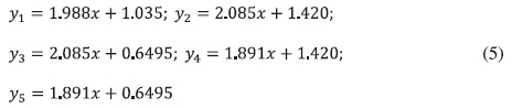
The resulting y₂and y₅boundary equations determine the widest range of error, i.e. confidence interval in graphic form for the whole model dependence. Thus, the value of x acquired from the model dependence also has its confidence interval Ax, which should also be taken into account. The measured value of y and the basic regression equation with its confidence intervals (Fig. 2.) makes it possible to determine an unknown x value (e.g. concentration).

 

 

3.1. Summary of Example from Fig. 2

1. The basic regression equation were determined via Origin.

2. The confidence intervals for a and b were determined with the use of s_a², s_b^%and t_Studentvalues.

3. The four border equations were determined. Basic equation and two external equations giving the widest confidence interval, were used.

4. For the measured value y_exp, the three values of x = 2.548; 2.245; 2.882 were determined from regression equation. This ultimately gives a range of x Є (2.245,2.882).

The overall form of a linear regression is given by Equation (6):

where Δa and Δb are respective confidence intervals (the ^ symbol indicates an estimated value read from the regression equation). If Aa = 0 and Ab = 0, we recognize a function dependence y = ax + b, which confirms that the function dependence is a special case of regression dependence, when all confidence intervals are zero.

The value read from the regression equation for given x,is always an estimated value labelled as ŷ. The y_i - ŷ_i difference, or precisely its square, is essential for the least squares method.

 

4. Least Squares Method

The above analysis was based on the Origin program without specifying the fact that it uses the least squares method to determine the regression curves (Figs. 1 and 2). This method is an optimization of a model dependence, where the criterion for optimization is to minimize the sum of model's deviations from experimental points, which can be visualized as a sum of square areas⁶ marked by dotted lines in Fig. 3, a solid line denotes model-experiment difference. Please note that the least squares method applied in analytical chemistry assumes no error in the concentration of the standards (x) and that the only variable is the signal (y).

 

 

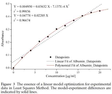
If a function y = f(x) is drawn through a set of measurement points x_i , y_i, then each x value will be matched with two values: measured (y) and estimated ŷ. The model, i.e. the regression equation, may be linear or curvilinear and expressed by an appropriate function.

For the linear regression y = ax + b, optimization criterion is to minimize the sum S(a,b):

where ŷ_i represents the estimated value based on the regression equation, and n represents the number of measured x points (in the case of multiple y measurements for each point x, average values should be used).

Equation (7) is a function of two variables, a and b. Determination of such function's minimum is possible by finding a point at which the partial derivatives for all its variables are equal to zero. Hence, the system of equations (8) and its rearranged form (9):

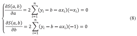
From the system(9) stemformulas forthe aand bcoefficients of a linear equation:

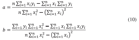
The method used is sensitive to presence of significantly deviating points in the dataset. Each of these will deviate outlined function toward its value, weakening the fit. Therefore, before using this method, any gross errors must be eliminated from the dataset, with the use of appropriate mathematical criterion.⁶

4.1. Least Squares Method - Example

Spectrophotometric method was used to measure samples containing known concentration of albumin (Bradford method) and glycine (ninhydrin method). The experiment was performed three times and the obtained experimental data are given in Table 2.

From formulas (1), (2) and (10) or faster using Origin, for albumin data we get:

Thus, the calibration curve equation is: y = 0.02205x + 0.0477.

The t(a,df) coefficient for the level of significance a = 0.95 and 9 degrees of freedom is 2.262 and the confidence intervals are as follows:

∆a = 2.262-1.850 · 10^-6 = 4.185 · 10^-6; Ab = 2.262-2.602 · 10^-4 = 5.886 · 10^-4. Therefore the final, rounded, linear regression equation looks like this:

The r²coefficient of Equation (11) equals 0.9667 which is a rather good but not the best result, as indicated by the second digit after the decimal point. This suggests the need to check other models.

On the other hand for glycine data, a = 83.26; b = 0.002650; s² =4.733·10^-5; s_a²= 0.2179; s_b² = 2.144·10^-5,which gives an equa-tion in the form of:

y = 83.26x + 2.650 · 10^-3.

For a = 0.95 and df = 7, t(a,df) = 2.365, thus calculated confidence intervals are consecutively ∆a = 0.5153; ∆b = 5.070 · 10^-5, which gives us the final equation:

For both considered examples, the values S₀², S_a², S_b² were calculated using Origin. Values of Da and Db, computationally simple, were calculated using an ordinary calculator.

For Equation (12), r² coefficient is equal to 0.9998. Its value being so close to 1 suggests a nearly perfect regression equation. However, in light of the current requirements of analytical journals, even almost perfect r² value does not constitute enough evidence of the suitability of the adopted model. It is still required to provide the results of additional statistical tests.

 

5. Lack of Fit Test^7,8

As was stated before, the r² coefficient cannot reliably indicate whether the adopted model is appropriate or not. To decide, statistical analysis should be performed on the adopted model. One of the statistical tests used for this purpose is Lack of Fit test, which can detect mismatches between the data and the adopted regression model.

Now, the regression model y_ij= ax_i+ b + ε_ij; {(x_i, y_ij ): i = 1,...,n; j = 1,...,c} is tested for the case where each of x_imatches with at least c = 3 y values (Table 2) for the data, where n is the number of measurements as previously used and c is the number of repetitions of the measurement for a given x. To consider that linear model fits the data, a null hypothesis H₀: = ax_i+ b must be maintained. To test it one has to calculate the sum of squares due to errors for the full (13) and reduced (14) models and then subtract them from each other (15).

Results obtained from Equations (13) and (15) should then be divided by their respective degrees of freedom (16), (17) which leads to Equations (18) and (19). The final result of this test is the F_LoFvalue (20).

To decide whetherto acceptorrejectthe nullhypothesis posed at the beginning of the test, the calculated F_LoFvalue (20) should be compared with the critical value F*_LoF (a; df_SSLF; df_SSEf_uU) taken from F distribution tables. If for the assumed level of significance a, the inequality F_LoF> F*_oFis true, the linearity hypothesis H₀: y_ij= a_xi+ b must be rejected.

5.1. Lack of Fit - Example

Lack of Fit test requires a minimum of three y values for each x. Therefore, in the example the original experimental values were used instead of the average ones (Table 2). The data were introduced consecutively into the formulas (13), (14), (15), next to (16), (17), (18), (19) and (20) giving results:

 

 

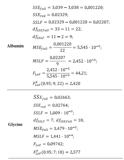
As one can see, the inequality F_LoF> F^#_LoF is true for albumin data. Thus, the null hypothesis of good linear model fit has to be rejected, and the alternative hypothesis stating that the linear model for the albumin data exhibits a mismatch should be accepted.

In the case of glycine data an opposite situation can be observed. F_LoF< F^#_LoF, thus there is no basis to reject the null hypothesis of linear model fitting the experimental data.

 

6. Classic Fisher-Snedecor Test^9,10

This test involves separate determination and comparison of the linear and quadratic effect's significance. The linear effect E_lin, which means that part of total variability of y, that can be described by the accepted model ŷ = ax + ", results from the expression (21)

where ȳ means the average value of the whole population of y. However, if the linear model is replaced with the quadratic one, i.e. ŷ = ax²+ "x + c, then the part of the total variability of the dependent variable, described by the parabola, results from expression (22), which is almost identical to Equation (21), with only one element different.

The quadratic effect E_qof the dependent variable's total variation is the part that can be further explained by replacing the linear model with the quadratic model. In order to obtain a formula for this effect, expression (21) has to be subtracted from expression (22) resulting in Equation (23):

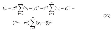
This test defines the significance of the both effects as a ratio of said effect to its residual variance. The value of the residual variance describes this part of the dependent variable's variability that remains after deducting the variability described by the independentvariable. Itcanbe calculated bydividingthe sumof deviations squares by the number of degrees of freedom. The number of degrees of freedom is equal to the number of independent variables minus the polynomial degree plus 1: df = n -(k + 1).

To ease the calculation, Equation (24) can be simplified by inserting an average value ȳ.

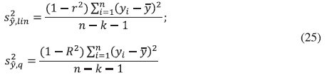
Having defined the concept of effects (21), (23) and residual variance (24), (25), the final test formulas for linear (26) and quadratic (27) effect significance can be obtained.

Lastly, the obtained linear and quadratic effect significances have to be compared with critical values F^# (a;1; n - k - 1) taken from F-distribution tables. If the significance of the effect is less than corresponding critical value, given effect should be considered as not significant. The more the F-value is greater than the F^#, the more significant the model is. Preferably F should exceed F^#by one or more orders of magnitude.

This test allows the possibility of having positive results for all tested models. Unlike other tests that give 'zero-one' like answers, the classic F-test results shows quantitative measure of each model's contribution in the data description. Therefore, despite its limited precision, it is a useful test in the evaluation of regression models.

6.1. Fisher-Snedecor Test - Example

The classic F-Snedecor test does not require multiple measurements for each independent variable. Moreover, in the case of multiple y data, values should be averaged beforehand. Therefore, both albumin's linear and quadratic regression models and their determination coefficients were obtained using the averaged data from Table 2.

At first, linear and quadratic effects and residual variance for both models were calculated. Afterward, the significance of both effects was determined.

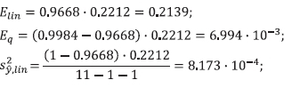
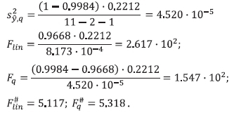
By comparing values of F_lin and F^#_lin it can be noticed that F_lin exceeds the critical value by two orders of magnitude. This indicates high importance of this effect and could be a basis for accepting the linear model. However, the value of quadratic model's significance exceeds its critical value by two degrees of magnitude as well. Hence the conclusion that the quadratic effect is an important contribution and cannot be ignored. This situation is a case where positive results are obtained for both effects.

For comparison, the same test was performed for glycine data (Fig. 5).

 

 

 

 

 

 

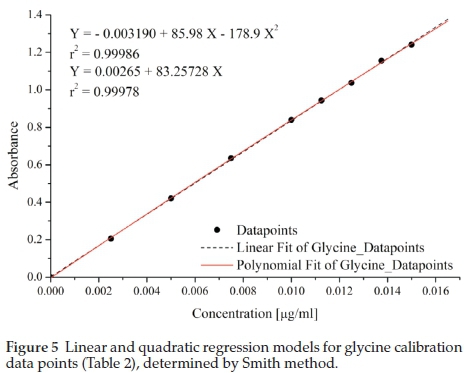
All the values were calculated same way as for albumin data.

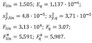
Significance of linear model F_linexceeds the critical value F^#_lin by four degrees of magnitude, which states greatly in favour of linear model. Moreover, the significance of quadratic model F_qis lower than its critical value F_q^#. Such results provide a strong basis for completely rejecting the significance of the quadratic model and using the linear regression model instead.

 

7. F-Snedecor Test Modification by IUPAC and Mandel

To prevent the possibility of an inconclusive the classical F-Snedecor test results, the International Union of Pure and Applied Chemistry (IUPAC) adopted its modified version based only on residual variances of both linear and quadratic model.¹⁰ Modified test checks whether the variance explained by the quadratic model is greater than the variance explained by the linear model. The null hypothesis H₀: 'the variance explained by the additional term is not different from the residual variance' is formulated. Thus, it is assumed that the quadratic model is not significant. Test equation has the form of Equation (28):

The modified test involves comparing the obtained value F_1UPAC with the critical value F^#_IUPAC(a; 1; n - 3). If the obtained value is greater than the critical value (exactly opposite to classic F-test), the null hypothesis has to be rejected in favour of the alternative hypothesis: the variance explained by the quadratic term is larger than the residual variance. That result would imply the need for a quadratic model.

The F_1UPACtest is simple and easy to understand. It does not consider directly the effect of degrees of freedom, which may call into question its usefulness in most cases where the number of calibration points is relatively low. For this reason, in 1964 a chemist and statistician, J. Mandel, suggested an improved version of the test. It was summarized as a comparison of the residual standard deviation of the linear model with that of the nonlinear model.¹¹ Unlike IUPAC, Mandel defined the F-test not as a subtraction of the variances of the two models, but as a subtraction of the sum of squares of the linear and quadratic fits, divided by the difference of their degrees of freedom.

Equation (29), can be simplified to a form similar to one specified by IUPAC (30):

As can be seen from (28) and (30), the only difference between the IUPAC and Mandel approach is that the latter one includes respective degrees of freedom. This results in a more detailed outcome, particularly in the smaller amount of data available, wherein the differences between both tests are the most visible.

Mandel test, as an IUPAC modification, compares the test to the same critical value F^#_IUPAC= F^#_M(a; 1; n - 3) and has the same condition for accepting or rejecting the null hypothesis.

Due to the use of degrees of freedom in Mandel's equation, it so happens that the result of the test differs sufficiently from IUPAC version. As a consequence, when both results are aligned with the same critical value, the obtained conclusions can be opposite. In such a situation one should accept the Mandel's F-test result as a more accurate one.

7.1. IUPAC and Mandel Tests - Example

To concretize the inconclusive results of the F-Snedecor test, both datasets (Table 2) were analyzed using F_IUPACand F_Mandeitests. The results of all F_IUPACcalculation steps are shown below.

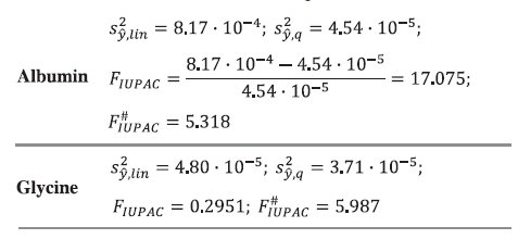
As it can be seen for albumin data, the F_IUPACvalue is three times bigger than its critical value F_IUPAC. This result indicates the need of quadratic model for albumin data.

In turn, test for glycine data showed no basis for quadratic model usage since F_IUPAC<< F^#_IUPAC. At this point one would say that the situation looks straightforward. However, F_IUPACtest, by not including the respective degrees of freedom in its equation, can give misleading results for some datasets¹² This is why even though the situation may look clear, a wise move is to conduct the more accurate form of this test, namely Mandel test. For the same set of data, Mandel test results are shown below:

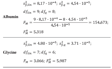
Since for albumin data F_M> F# and for glycine data F_M< F#, the conclusions of Mandel and F_IUPACtests are alike. This confirms that albumin data requires quadratic model to be used while there is no need to do that for glycine data.

 

8. A Summary of Respective Statistical Tests

For clarity, the results of the four tests application were gathered in Table 3.

As shown in Table 3, for glycine data the linear model was consistently confirmed by all four test results and there is no justification for using the quadratic model.

Albumin data do not give such consistent results. Only three of four conducted tests, namely Lack of Fit, F_¡UPACand Mandel tests,

stated in favour of quadratic model while classic F-Snedecor test showed a draw. Even though this is enough to indicate the need for quadratic model, as the linear one is not sufficient in case of this dataset.

As it can be seen above, the F_Mvalue for albumin is considerably higher than F_IUPACfor the same data. This shows how big of a difference makes including degrees of freedom, mainly for the cases with fewer data points. In such cases, where values given by both tests are close to the test's critical values, one has to evaluate the numerical values obtained from the tests, taking their force into account. Also, one could consider redoing the calibration procedure and adding more experimental points.

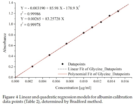
Now that the statistical tests are done and the quadratic model was chosen, one could question how greatly the choice of the model impacts the outcome of an experiment that utilizes it to get results. To show that we will once more use albumin data (Table 2, Fig. 4), but this time we will be using the model rather than creating it. Albumin data points were obtained experimentally, hence their (x, y) values are certain. Therefore, one can compare those values with the x values obtained from both models to see how much a calculated value can deviate from an actual, measured value. The results are shown in Table 4.

One can easily see that the values attained from linear model deviate in general from the actual values by almost a full unit of concentration. Therefore using this model could lead to a significant error in the calculated results. On the other hand, the values obtained from the quadratic model deviate in general just by a quarter of a full unit of concentration, which means that this model is about four times less likely to cause result errors.

As much as the quadratic model is more precise in this situation it also comes with some downsides which cannot be forgotten. To properly use this regression model, one has to remember that its sensitivity is not constant along the curve as it is for linear model. Its value is equal to regression model's first derivative ^dAbs/_dC= -14.27 · 10^-4x + 0.03632. This can be easily shown by testing the model for small absorbance changes. For small absorbance range, e.g. from 0 to 0.1, a little change, DAbs = 0.05, corresponds to an equally small change, DC = 1.408 in calculated concentration, whilst the same change DAbs = 0.05 for final absorbance range from 0.400 to 0.500 corresponds to a much bigger change, DC = 4.806. It is visible that at the end of the calibration curve the model is four times less sensitive on measured factor (Abs) than at its beginning. As an effect, expected C result, obtained from final range of the model, is loaded with much greater error. If possible, one should work in the part of quadratic model where the sensitivity is still fairly high what can be achieved, e.g. by respective dilution. It can be assumed that said region is maintained up to the point where the respective derivative is greater than the linear dependence model's slope, i.e. 0.02205. The critical point obtained by simple calculation is at C = 9.948 »10 mgmL^-1, which remains in good agreement with an intuitive observation (Fig. 4). It means, that in considered case one should use the region up to C = 10 µgmL^-1 to obtain reliable results.

In conclusion it can be said that the presented and applied four statistical tests are useful and necessary. They also, through positive feedback, lead to an improved experimental procedures as they oblige researchers to pay more attention to the layout of their experiments. The validation of the adopted regression model adequacy should be based on several rather than one of the provided statistical tests which give a complete picture of reality. All of the discussed tests can be easily done using only basic spreadsheet programs or even just by using a calculator. Therefore, the presented statistical analysis of linear and quadratic regression models is commonly available and should be performed whenever it is possible.

 

Abbreviations

Symbol Meaning

a Slope of linear dependence

b Intercept of linear dependence

s₀ Standard deviation

s_a Standard deviation of a

s_b Standard deviation of b

s² Residual variance

B Slope in ORIGIN software output

A Intercept in ORIGIN software output

a Level of significance

t (a, df) t_Student coefficient

df Degrees of freedom

n The number of x values

c_i The number of y_irepetitions for given x

E_lin, E_q Linear and quadratic effects

F_lin, F_q Fisher-Snedecor test values

E_Lof Lack of Fit F-test value

F_IUPAC IUPAC F-test value

F_M Mandel's F-test value

SSE_red Sum of squares due to reduced model errors

SSEf_ull Sum of squares due to full model errors

SSLF Sum of squares due to lack of fit

MSEf_ull Mean squares due to full model errors

MSLF Mean squares due to lack of fit

r² Determination coefficient of linear model

R² Determination coefficient of quadratic model

^ Symbol of estimated value

^- Symbol of mean (average) value

^# Symbol of critical value

 

References

1 J. Van Loco, M. Elskens, C. Croux and H. Beernaert, Linearity of calibration curves: use and misuse of the correlation coefficient, Accred. Qual. Assur, 2002, 7, 281-285.         [ Links ]

2 Analytical Methods Committee, Is my calibration linear?, Analyst, 1994, 119, 2363-66.         [ Links ]

3 L. Brüggemann, W. Quapp and R. Wennrich, Test for non-linearity concerning linear calibrated chemical measurements, Accred Qual Assur, 2006,11, 625-631.         [ Links ]

4 J.J. Faraway, Practical Regression and Anova using R, Johns Hopkins Bloomberg School of Public Health, 2002, http://www.biostat.jhs-ph.edu/~iruczins/teaching/jf/ch3.pdf        [ Links ]

5 J.R. Taylor and A. McGuire, ed., An Introduction to Error Analysis, the Study of Uncertainties in Physical Measurements, 2nd edn., University Science Books, Sausalito California, USA, 1997.         [ Links ]

6 K. Doerffel, Statistik in der Analytischen Chemie, VEB Deutscher Verlag für Grundstoffindustrie Leipzig, 1984, 181-182.         [ Links ]

7 J. Wei and D. Paul, StatWiki 2015, UC Davis GeoWiki by University of California http://statwiki.ucdavis.edu/Regression_Analysis/Sim-ple_linear_regression/Test_for_Lack_of_Fit        [ Links ]

8 L.C. Rodriguez, A.M.G. Campana and J.M.B. Sendra, Statistical estimation oflinear calibrationrange, Anal. Lett, 1996,29(7), 1231-1239.         [ Links ]

9 J. Czermiñski, A. Iwasiewicz, Z. Paszek, A. Sikorski, Statistical Methods for Experimental Data Processing (Metody Statystyczne w Doswiad- czalnictwie Chemicznym), 2nd. edn., Polish Scientific Publishing House (PWN), Warsaw, Poland, 1974 (in Polish).         [ Links ]

10 K. Danzer and L.A. Currie, Guidelines for calibration in analytical chemistry. Part I. Fundamentals and single component calibration (IUPAC Recommendations 1998), Pure Appl. Chem, 1998, 70(4), 993-1014.         [ Links ]

11 J.M. Andrade and M.P. Gomez-Carracedo, Notes on the use of Mandel's test to check for nonlinearity in laboratory calibrations, Anal. Methods, 2013, 5, 1145-1149.         [ Links ]

12 M. Zaręba, P.T. Sanecki and R.I. Rawski, Simultaneous determination of thimerosal and aluminum in vaccines and pharmaceuticals with the use of HPLC method, Acta Chromatography, 2015, DOI: 10.1556/1326.2016.28.3.2, to be published in issue no. 3 (September) / 2016.         [ Links ]

13 B. George and E.P. Papadopoulos, Heterocycles from N-ethoxy-carbonylthioamides and dinucleophilic reagents, J. Org. Chem., 1977, 42, 441-43        [ Links ]

 

 

Received 25 February 2016,
Revised 24 June 2016,
Accepted 29 June 2016.

 

 

* To whom correspondence should be addressed. E-mail: psaneckl@prz.edu.pl

 

 

Appendix

Additional Materials

Excel spreadsheets used for all of the applied tests are available on request by e-mail.

Software Alternatives

There is a possibility to substitute both Origin Pro and MS Excel with free open source programs, receiving the same output values. Instead of Origin Pro and MS Excel one can easily apply following programs:

• SciDaVis - https://sourceforge.net/projects/scidavis/

• Libre Office - http://libreoffice.org/download/libreoffice-f-resh/