TECHNICAL PAPER

 

Systemic efficiency and capacity: A vital combination in the design of dedicated rail freight projects in Southern Africa

 

 

F J Mülke; J H Havenga; J van Eeden

Correspondence

 

 

---

ABSTRACT

A model was composed that integrated demand for railway services, systemic capacity design of production factors, operating efficiency, and the financial viability of the designed railway operations of a dedicated rail freight project. The design model incorporated efficiency measures essential to successfully developing new railway systems.
The investment in rail infrastructure concerning the geometric parameters and their effect on the project's viability was deduced. A relationship between the geometric layout of track alignment and the hauling process of freight was determined. Results from simulation work to ascertain the operating efficiency informed the design of train-crossing capacity. The effect of inefficiencies on the performance of the production factors and the influence thereof on the rail tariff and the internal rate of return was determined.
The design model covered the range of demand from low volumes of dedicated freight to the advent of heavy-haul operations, and will find its application in cases of new green-field projects. The design parameters applied in sub-models were correlated with the results of field tests and individual new railway projects undertaken in Southern Africa. The results of the effect of systemic operating efficiency on the capacity of the rolling stock fleet were illustrated.

Keywords: demand, capacity, systemic operating efficiency, tariff rate, internal rate of return

---

 

 

INTRODUCTION

Of late, mining ventures have been developing new projects in Southern Africa, and opted to construct and operate their privately owned rail logistics supply chain, linking their mines in the hinterland with a port. Embarking upon these pit-to-port projects emphasised the need to develop a model to design, integrate and optimise the production factors of rail service. In response to this need, a design model was developed to incorporate the design and capacity creation of capital-intensive production factors, the systemic operating efficiency, and the associated returns to scale of a dedicated rail freight system.

This paper attempts to explain the development of an integrating design model that will correlate the production factors' effective and productive capacity design with the efficient performance level of the systemic operations driven by demand. The systemic operating efficiency is expressed in terms of the actual cycle time, also referred to as the turnaround time (TAT) of a railway system and termed as a factor of the most time-saving TAT. An essential feature of the design model entailed the simulated effect of systemic operating efficiency on the capacity deployment of the rolling stock and the integration with the rail infrastructure alignment.

The sub-models determined the capex and opex of the design of the production factors. These were integrated into the financial model to produce the project's final rail tariff rate and internal rate of return (IRR).

Finally, applying a dashboard of the design model produces financial results that will ensure a closer valuation of a railway project to its final value at an early phase of its development.

 

OBJECTIVES OF THE RESEARCH

The primary objective of this paper is to give an exposition of the development of an integrating design model that will correlate the effective and productive capacity design of the production factors with the efficient performance level of the systemic operations driven by the demand depicted in mega tonnes per annum (Mtpa), for a new greenfield dedicated rail-freight project.

Sub-objectives of the development of a design model

Achieving the primary objective required the attainment of the following sub-objectives:

■ Sub-objective 1: Establish the interrelationship between the macro geometric layout of the linear track structure and the earthworks volumes.

■ Sub-objective 2: Determine the correlation of the haulage performance of the rolling stock related to the macro geometric track alignment and the demand.

■ Sub-objective 3: Determine the effect of levels of systemic operating efficiency on the capacity of the rolling stock.

■ Sub-objective 4: Determine the effect of the capacities and processes on the capex and opex, the rail tariff rate and the IRR of a new dedicated rail freight project (Kay 1976; Drury 2009).

 

METHOD OF DEVELOPING THE SUB-MODELS INTEGRATED INTO THE DESIGN MODEL

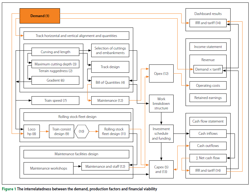
The approach to developing the integration process of the sub-models into the design model and the analysis of the interrelated-ness of the production factors of a new railway system are shown in Figure 1.

The linkages indicate the interrelatedness produced by the demand as the primary driver of the design algorithm (Leonard 1986).

Realising sub-objective 1 (the establishment of the interrelationship between the macro geometric layout of the linear track structure and earthworks volumes) entailed:

■ Determining the demand (1) as the independent variable that drives the selection of variables in the design processes.

■ Observing the undulating topography (2) determines the selection of the conceptual maximum depth of the cuttings (3) and the minimum radius of the curving of the trackwork, thereby dictating the resultant earthworks cost.

■ Structuring the Bill of Quantities (4) based on the cutting depths, length and number of cuttings and the rail route length, defining the extent of the earthworks capex (5).

■ Determining the macro geometrics of the line, length and steepest gradient (ruling grade) (6).

Pursuing sub-objective 2 (the correlation of the haulage performance of the rolling stock related to the macro geometric track alignment and the demand) was determined as follows:

The demand is a moderating variable for the train consist design. In conjunction with the ruling grade (6) and the summit balancing speed (7), it informed the solving of the number of locomotives with specific power characteristics (8) to haul the train consist (9). The power of the selected locomotive type is a dependent variable interrelated to the demand.

Reaching sub-objective 3 (the effect of levels of systemic operating efficiency on the capacity of the rolling stock) was determined as follows:

■ The systemic operating efficiency factor (10) is a moderating variable in determining the rolling stock fleet size.

■ The demand is divided by the train consist's payload (9) to solve the required fleet size of locomotives and wagons (11).

■ The required rolling stock fleet size (11) determines the capex of the haulage operations and support processes. Its performance on the macro geometrical track layout determines the opex, of which the fuel consumption forms the major cost element.

Attaining sub-objective 4 (the effect of the capacities and processes on the capex and opex, the rail tariff rate and the IRR (Kay 1976) of a new dedicated rail freight project) was integrated into the design model, namely:

■ The maintenance of the trackwork (12) and rolling stock (12), including the operational costs for fuel, lubricants, and train crews (12), produced the opex of the railway system (Parajuli 2005).

■ The investment in the rail infrastructure, the rolling stock fleet, and the ancillary facilities, e.g. maintenance workshops, informed the capex (13) in the cash flow analysis.

■ The revenue of the operations was calculated using the product of the demand and the rail tariff rate. The rail tariff rate controls the IRR (14) and is determined in an iterative method by the opex of the production factors and the demand (1) to produce positive net cash flow.

 

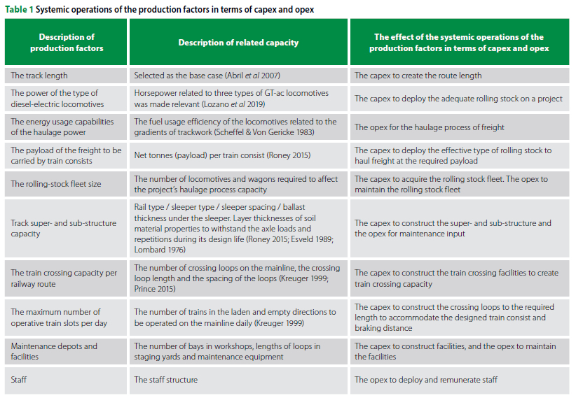
CAPACITIES OF A RAILWAY SYSTEM

The UIC (International Union of Railways) (UIC 2015) stated that, "A unique true definition of capacity is impossible. Rail infrastructure capacity depends on the way it is utilised", after which Sameni (2012) remarked that capacity "... is a trade-off between the number of trains, heterogeneity, and average speed". The capacity design of a new railway project primarily entails determining the conveyance capabilities of the production factors linked to demand (Sameni 2012).

The selection of capacities (Abril et al 2007; Boysen 2012a; Lindfeldt 2015) of the railway systemic sub-systems that had been integrated at haulage performance levels of the demand is shown in Table 1.

 

THE MACRO GEOMETRIC LAYOUT OF THE LINEAR TRACK STRUCTURE RELATED TO EARTHWORK VOLUMES

The selection of the macro geometrics of the alignment of the rail route (i.e. the minimum radius of curves, the ruling grade, the minimum of trackwork between grade changes and the crossing loop spacing) is related to the demand of the railway venture. From a cost-effective perspective, the ruling grade and curving of the horizontal alignment impact the creation of earthworks volumes and the cutting configurations.

The quantification of volumes of cuttings versus cutting depths for cutting lengths

The earthworks volumes sub-model quantifies the relationships between the capital cost for specific cutting configurations and the linear track work, allowing the trading off against the train hauling performance and the variable cost of freight haulage.

In the case of projects with high demand values, the degree of curvature can be reduced as well as the ruling grade, resulting in deeper cuttings becoming feasible.

The relationship between the depth of a cutting and the unit volume/m is indicated in Equation 1.

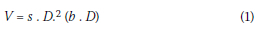
Where:

V is the unit volume (m³/m)

s is the side slope of the cutting (ratio)

b is the width of the cutting floor (m)

D is the maximum cutting depth (m).

The spectrum of several formations of cuttings was grouped in classes of dimensions en route sourcing the fill material of the sections of embankments, which was configured in a sub-model (Skempton 1996).

The quantities of cuttings were calculated using Simpson's Third Rule (Dhali et al 2019). The volume of cuttings versus the maximum cutting depths for selected cutting lengths is shown in Figure 2.

 

 

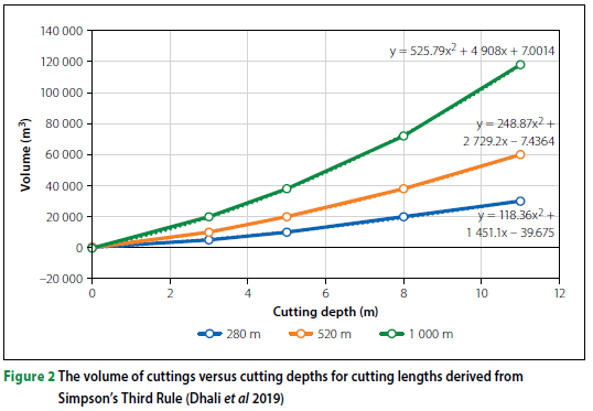
The cut-to-bank and borrow-to-bank quantities were deduced, including all ancillary costs of related earthworks items, and priced in a Bill of Quantities, which informed the capex in the design model (Duffy 2018; Preston 1992; Dhali et al 2019).

 

PARAMETERS FOR THE DESIGN OF THE TRACKWORK SUPERSTRUCTURE DESIGN

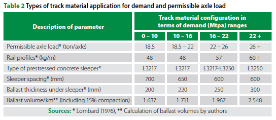
The parameters for the track superstructure design were based on the ramp-up of demand ranges and, consequently, the associated permissible axle loads. The composition of trackwork material in the track-work sub-model was linked with ranges of axle loads, as shown in Table 2.

 

 

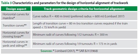
Characteristics and parameters for the design of the alignment of trackwork

The characteristics and parameters which were applied in the design of the horizontal alignment of a greenfield section of new trackwork in Southern Africa are set out in Tables 3 and 4.

 

 

 

 

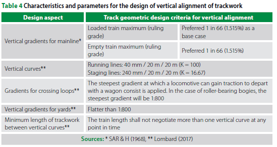
The characteristics in Table 4, read in conjunction with Table 3, were applied in the design of the vertical alignment of the trackwork.

A summary of the track material and construction items composing the Bill of Quantities is described in Table 5.

 

 

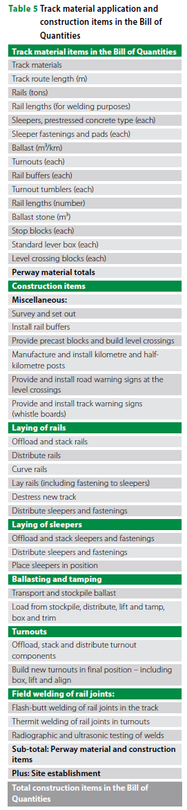
The composition of the Bill of Quantities for mainline trackwork, crossing loops, and yards was developed by obtaining its trackwork quantities as follows:

■ The mainline track length, based on the rail route length, was adjusted with a stagger due to the topographic undulation effect (Kweon & Kanade 1994; Riley et al 1999).

■ The number of turnouts was informed by the number of crossing loops and the number of staging lines in the yards.

■ The lengths of the crossing loops and staging lines were deduced from the train length and braking distance of the trains.

■ The number of staging lines in yards was related to the demand and the number of train sets.

The trackwork investment estimates informed the cashflow projections in the financial model.

Cost relationship between the macro geometric layout of the linear track structure and earthworks volume

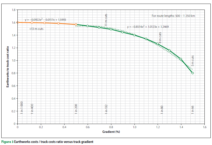
To determine the ratio of cost between the macro geometric layout of the linear track structure and earthworks volumes, a set of parameters was applied in the case of the steepest gradient of a railway line, namely 1 in 66. In this regard, the gradient and maximum cutting depth for lengths of track route and the ratio between earthworks and trackwork costs were determined and are shown in Table 6.

 

 

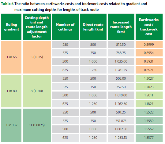
As a form of augmenting the range of parameters, the maximum cutting depths for rail routes were paired to corresponding ruling gradients, as shown in Table 6. Route lengths were adjusted by adding 2.5% in the case of the 1:66 ruling grade, 1.0% for the 1:80 ruling grade and 0.25% for the 1:132 ruling grade. The ratio of earthworks cost to trackwork cost for the route lengths varying from 500 km to 1 250 km is shown in Table 6 and illustrated in Figure 3.

The ruling grade, as the independent variable, was plotted in Figure 3 on the x-axis, and the ratio of earthworks cost / trackwork cost was plotted as the dependent variable on the y-axis.

■ The maximum gradient for trackwork was selected as 1 in 66 (1.51515%) and was paired with 5 m cutting depths.

■ The lengths of the cuttings were considered in the cases of the three types of ruling grades with maximum cutting depths of 5 m, 8 m and 11 m, ranging from 280 m to 1 000 m.

■ The maximum cutting depth of 13 m was selected. In practice, a railway cutting with a depth of 13 m was assumed to require "benching" by stepping the side slopes at 6 m depth, thereby creating "a cutting within a cutting" (Rauch n.d.).

The equation reflecting the interrelated ratio of earthworks costs / trackwork costs versus ruling gradients for cutting depths up to 13 m was determined by the authors utilising a quadratic fit as shown in Equation 2.

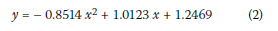
Where:

y is the ratio of earthworks cost / trackwork cost

x is the track gradient (%).

The ratio of earthworks cost / track cost versus track gradient in Figure 3 shows that earthworks costs equal the trackwork costs at a gradient of approximately 1 in 72 (1.39%). For grades flatter than 1:200, with cutting depths shown in Figure 3, the earthworks costs exceeded trackwork costs significantly. The ratio of earthworks versus trackwork costs remains constant for gradients flatter than 1 in 200 due to the limitation of 13 m as the maximum cutting depth (Rauch n.d.).

 

THE HAULAGE PERFORMANCE OF THE ROLLING STOCK

The haulage performance of the train consist was based on the resistive forces acting on the train consist and the train summit speed (Bureika 2008).

The design of the train consist

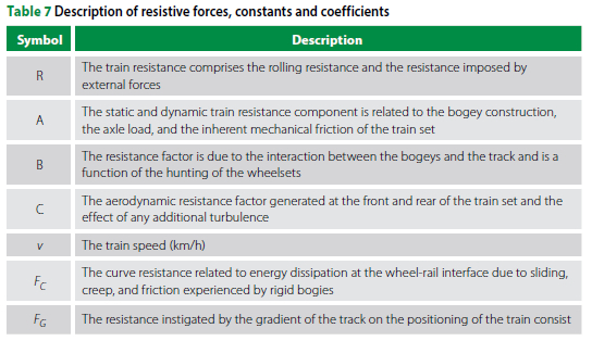
Davis (1926) formulated the relationship between the rolling resistance exerted on a locomotive during acceleration and attaining line speed. The resistive force (R) that opposes the motion is created by the friction of the axle bearings, the resistance between the wheels and the rail, air resistance, and external forces, as shown in Equation 3 (Mallery 2010). The external forces acting on the train's movement are created by the gradients of the trackwork and its curvature (Coals to New Castle 2017).

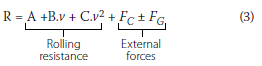
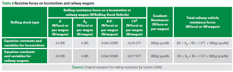
The resistive forces, constants and coefficients are portrayed in Table 7.

 

 

Szanto (2016) published test results of the resistive forces on railway vehicles on the Hunter Valley and Pilbara lines in Australia. The values of the constants and coefficients (A, B and C) derived for narrow-gauge rolling stock, are shown in Table 8.

The gross mass (M) for GT38ac, GT42ac and GT46ac type locomotives with axle loads of 18.5 tons, 20 tons and 26 tons gross, respectively, were applied in the hauling sub-model. The train speed (V) of 20 km/h at the summit of the line, used by Szanto (2016), was adopted in the design of the train consists. The external force due to the gradient (grad %) and the gravitational acceleration (g) was included in the compilation of the total railway vehicle resistance force.

 

Resistive forces due to the curvature of trackwork

Scheffel and Von Gericke (1983) designed and developed a self-steering bogie with near-zero curve resistance and virtually no side-wear effect on rails and bogie wheels. In creating a design model, it was assumed that the rolling stock would be fitted with Scheffel-type bogies (Scheffel & Von Gericke 1983; Ball 2016), and consequently the value of the curve resistance force (F_c) was considered negligible (McGonigal 2006).

 

The design of the train consist

The available drawbar horsepower of a locomotive was determined by solving Equation 4 (Indian Railways Institute n.d.):

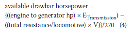
Where:

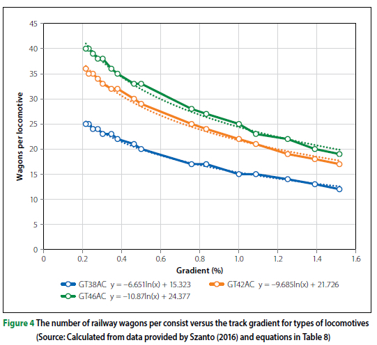
■ The power of the GT38ac, GT42ac and GT46ac type locomotives is 2 000, 3 000 and 4 300 hp, respectively

■ Transmission efficiency (ET_ransmission) for a GTac type locomotive is 0.94 (Indian Railways Institute n.d.).

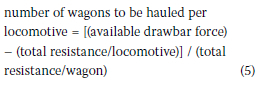
The number of laden wagons that a locomotive can haul on a specific gradient with a summit speed (V) of 20 km/h was calculated by dividing the available drawbar force by the resistive force per railway wagon in Equation 5 (Szanto 2016):

The relationships between wagons in the consist versus the gradient for types of locomotives were derived from the equations reflected in Table 8 of which the results are shown in Figure 4.

 

 

The haulage design was based on the configuration of train consists and the required number of train trips per year, based on the TAT (turnaround time) and the restriction of the number of train slots per day to convey the required demand.

The design of the rolling stock fleet size

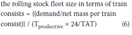
"The main drivers in determining the rolling stock fleet size of a new railway system for dedicated rail freight (from pit-to-port) are the demand and the TAT" (Mülke et al 2021), as per Equation 6:

Where:

■ T_productive represents the number of productive days of haulage by the railway system during the year

■ TAT is the turnaround time (hours).

"The additional number of wagons and locomotives required at the reduced efficiency levels represented the rolling stock required to operate at the inefficient level of the system to deliver the target demand" (Mülke et al 2021).

Equation (6) was further developed to reflect the rolling stock fleet size concerning the number of locomotives and wagons, which was solved by applying Equation 7:

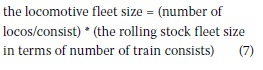
The solving of the wagon fleet size can be determined by applying Equation 7 and substituting the number of locomotives/consist with the number of wagons/ consist.

The capex of production factors associated with the hauling process was based on the results produced utilising the dashboard process depicted hereunder.

 

EFFECT OF SYSTEMIC OPERATING EFFICIENCY ON THE CAPACITY OF THE PRODUCTION FACTORS

Systemic operating efficiency (E_TotEff), as it relates to the railway environment, refers to the lack of waste (Carr 2016; Prince 2015). The inefficiency of a railway operating system stems from wasted time and, specifically, the resulting increase in the turnaround time (TAT) to affect an increase in production factors (Abril et al 2007; Aikaterini 2010; Grosskopf 1993; Jondrow 1982).

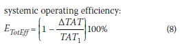
The TAT encapsulates all the time-related processes to load a train, operate it through the network, stage and offload the train, stage the empty train, and return it to its origin (Dutton & Mülke 2017). The systemic operating efficiency can be determined by Equation 8:

Where:

∆TAT = TAT₂ - TAT₁

E_TotEff is the systemic operating efficiency expressed as a percentage < 100%

TAT₂ is the TAT at the inefficient performance level

TAT₁ is the TAT at the efficient or design performance level or the efficient reference base case.

The systemic operating efficiency was determined by simulating scenarios for variations in average train speed versus a range of delayed-release times of trains from the inland departure point. The constraining factors included the late release of laden and empty trains into the mainline.

The results of the delayed train crossing time versus the average train speed for levels of systemic operating efficiency are plotted in Figure 5. Notably, the E_TotEff ranged between 68% and 100%.

 

 

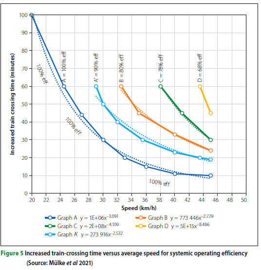
The late departure of trains had a diminished effect on the systemic operating efficiency of the system. It had a more significant impact on the system's performance in the case of fast-moving trains and short dwell times in the endpoint, resulting in the densification of train slots and an increase in the randomness of train movements. A delay buffer time of 25 minutes was conceded in the scheduling of trains and correlated with the Kuys et al report (2017).

The efficiency of the application of the fleet size to haul the annual demand compared with the systemic operating efficiency is shown in Table 9.

 

 

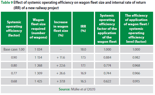
Comparing the wagon fleet sizes in the case of the systemic operating efficiency decreasing from 1.00 to 0.68, the wagon fleet size increased by 37.8%, and the IRR reduced correspondingly from 18.0% to 16.5%.

Applying the systemic operating efficiency factor in the design of train-crossing capacity

The longest section between crossing loops determines the capacity of a single railway line. The train-crossing capacity of a single line (C) is shown in Equation 9 and is a function of the systemic operating efficiency E_TotEff:

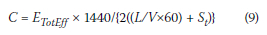
Where:

C is the train-crossing capacity expressed in the number of laden train slots per 24 hours

V is the average speed of the trains operated between the crossing loops (km/h)

L is the spacing extent between the crossing loops (km)

S_t is the train-crossing time (minutes) in the crossing loop, based on the dwell time of the empty train to allow the laden train to pass and clear the loop

E_TotEff is the total systemic operating efficiency of the loading, unloading, crossing and running of trains.

The spacing between the crossing loops (L) for variations in average train speeds and the systemic operating efficiency was solved using Equation 9. The calculation results of the number and length of crossing loops as a function of the train length, the braking distance and train speed were incorporated in the haulage sub-models as a sub-process of the design model and informed the capex (Zuan 2007; The Mathematical Association (UK) 2004).

 

THE DESIGN MODEL

The design model embodies the demand as the determinant for railway services in design processes to ascertain the capacities of the production factors.

The demand-driven systemic design

The demand can vary in ramp-up rate, the level of steady-state and prospects of increasing the project life at a later stage of the project life cycle.

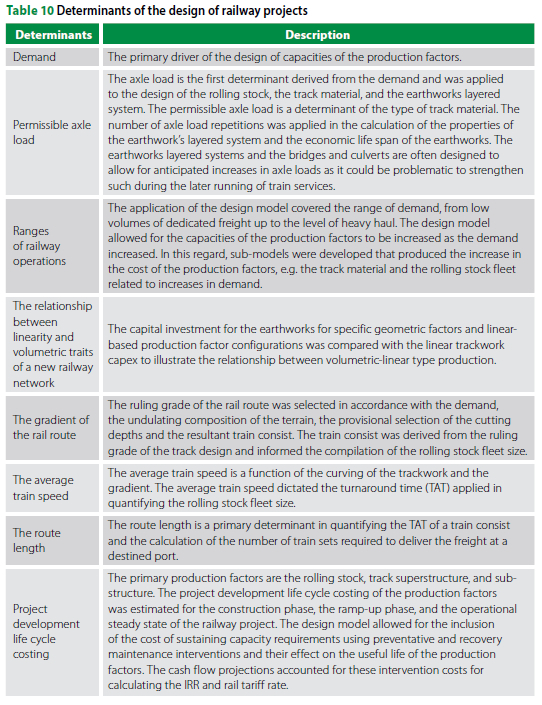
The determinants of the design of the capacities of the railway project were considered paramount in compiling the interactive sub-systems of the design model and are summarised in Table 10.

 

 

The design model as an algorithm

Cormen et al (1990) described an algorithm as a "sequence of computational steps that takes input values and transforms them into output values".

The objective of the compilation of an algorithm, holistically referred to as the design model, was to construct the interlink-age between sub-processes in sub-models. The dashboard enabled the selection of input capacities, which then produced the capex and opex of the following main processes:

■ The rail infrastructure

■ The train hauling process

■ The train operations

■ The financial modelling.

The input to the sub-models and the design assumptions formed steps in the algorithm to compute the two ultimate output parameters, namely the rail tariff rate (US dollar / net tonne-km) for a given IRR.

The methodology of using the dashboard entailed the following process:

■ Determine the demand.

■ Determine the input to the rail infra-structure sub-model in terms of the topo-graphical layout of the terrain en route:

■ the staggered length of the line

■ the ruling grade

■ the depth of the cuttings associated with the selected gradient

■ the number of cuttings on the line. The resultant output of the rail infrastructure sub-model comprised the volumes of earthworks creating the input to the Bill of Quantities and developing the capex value of the earthworks.

The route length and demand produced the input to the trackwork Bill of Quantities informing the compilation of the capex of the rail infrastructure.

Subsequently, the following train performance requirements were selected:

■ The appropriate locomotive type for the demand range in which the operations were conducted

■ The number of trains per day to be compared with the system's restriction of the number of train slots or trains per day.

As output, the rolling stock fleet size was derived from the configured algorithm using the dashboard. The rail tariff rate was ascertained by realising the required IRR of 20% (Luiu et al 2018).

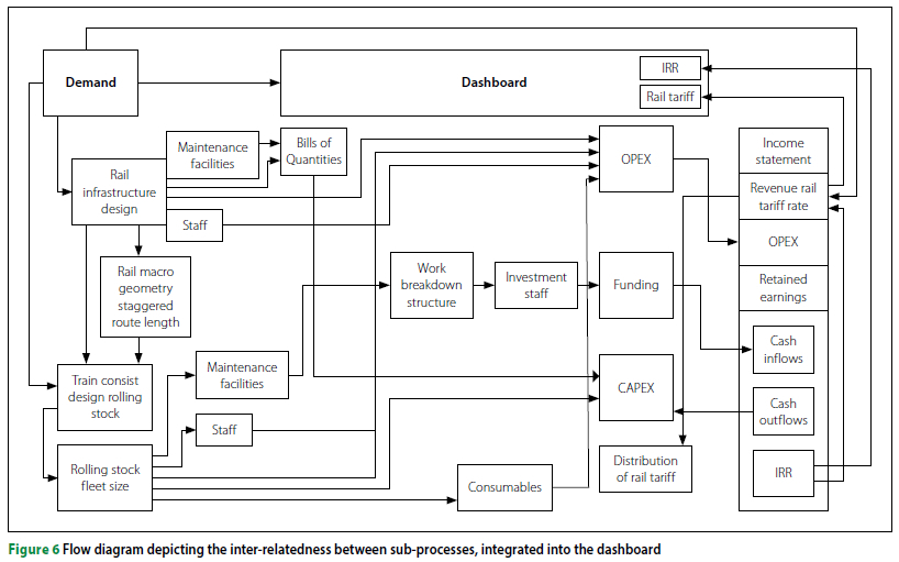
The logic of integrating the input of various sub-processes in the dashboard is illustrated in the flow diagram Figure 6.

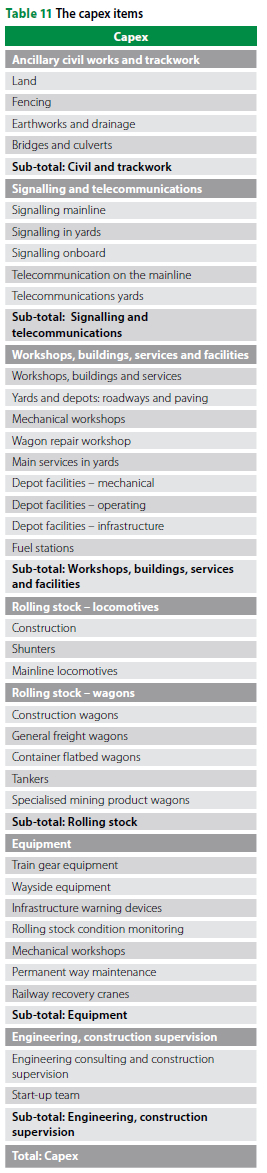
In addition to the requirements to assure the performance of the rolling stock fleet size, the demand determined the capacities, and consequently the capex of the production factors as set out in Table 11 (Ghoreishni 2019).

 

 

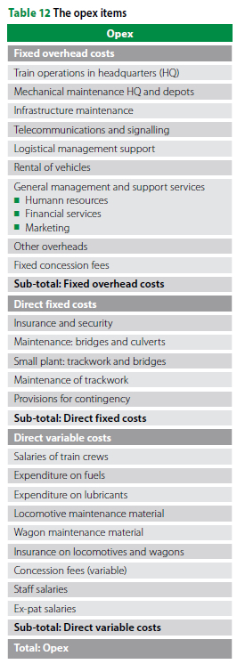
Opex estimate for the project

The typical opex items of a dedicated rail freight project are listed in Table 12.

 

 

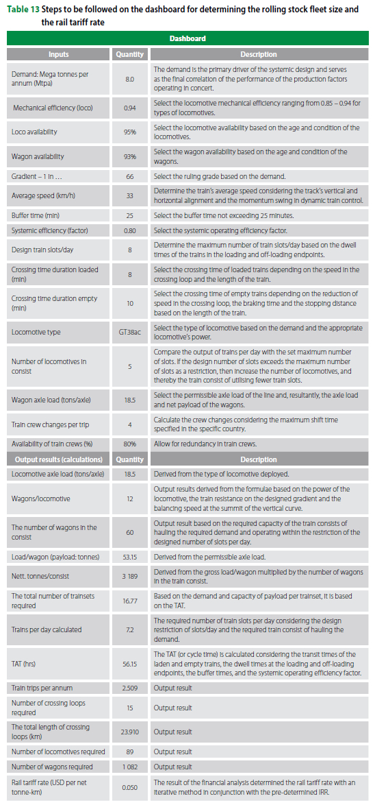
The construct of the dashboard reflecting the integrated process for determining the rolling stock fleet size and the rail tariff rate for a set IRR is shown as an example in Table 13.

 

 

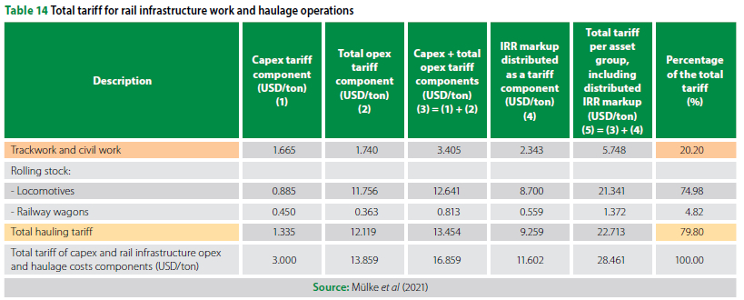
Finally, the cost of creating capacities of the locomotive and wagon fleets was computed as variable capex, varying with the demand, and adjusted following the effect of the level of systemic operating efficiency. An example of the results of a specific scenario of input values that rendered output results is shown in Table 14.

Mülke et al (2021) stated: "A cost structure analysis indicated that the investment cost of rail infrastructure can comprise 20.2% of the rail tariff and that the rolling stock and haulage costs can comprise the remaining 79.8%. The haulage costs mainly consist of variable capex and opex over the short and long term (Parajuli 2005). In contrast, the rail infrastructure costs consist of investment in the track length, the number and lengths of crossing loops and the ancillary civil works"

 

RESULTS

The rail tariff distribution of train consist hauled by types of locomotives

The rail tariff of the haulage process for the deploying of the types of locomotives GT38ac, GT42ac and GT46ac, was derived from the application of the algorithm expressed in selecting the variables in the dashboard.

The capacities of the production factors were determined for the various demand levels and informed the investment schedule and the cash flow statement. Finally, the capacities of the locomotive and wagon fleet sizes were computed as variable capex, varying with the demand, and adjusted by the level of systemic operating efficiency.

In Figure 7, the tariff rate versus demand for types of locomotive traction was plotted for a systemic operating efficiency factor of 0.90 and variation in route lengths.

 

 

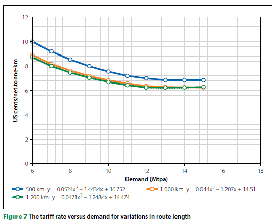
The rail tariff rate decreased with the increase in route length and was attributable to the effect of earthworks costs incurred at the two endpoints. The product of the route length and the rail tariff rate rendered the tariff expressed in USD/ tonne, which increased with the increase in route length.

The long-term and short-term average cost curves

The concept of economies-of-scale refers to the potential of using the unused capacity of a railway system at marginal increases in input cost. The use of track-carrying capacity (train slots/day) that is available for the increased haulage of additional volumes is an example of the use of "economies of scale" (Samuelson 1970). The effect of economies of scale and dis-economies of scale is calculated during the quantification of the long-run average cost curve (LAC) (Pettinger 2019; BCampus Open Publishing 2019; Chen 2007). This aspect was contained in a cash flow projection, which formed the basis of the design model for determining the rail tariff rate and the IRR (Luiu et al 2018).

As an increasing number of trains absorb the capacity of the fixed assets, the lowest average haulage cost at that point of haulage activity is reached, after which it will increase when additional capacity is required. The new level of capacity creation can be in the form of longer trains with additional locomotive power, which would entail additional capital investment. The next stage of capacity increase would involve increasing the axle loads of the rolling stock. In such a case, further capital investment would be required in the track superstructure and the carrying capacity of the rolling stock, e.g. heavy-haul vehicles (Denley 2018; Tourney & Fröhling 2015).

The cost productive indicator net tonne (CPINT)

A cost-productive indicator net tonne (CPINT) was compiled based on the variables in Equation 10, namely:

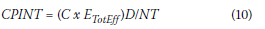
Where:

CPINT is the cost productive indicator of net tonne hauled

C is the total average cost (USD/tonne)

D is the demand (Mtpa)

E_TotEff is the systemic operator efficiency factor

NT is the production activity indicator represented by the payload of the wagon consist (net tonne).

The payload of the wagon consist is an indicator of the train unit's conveying capacity based on the axle load as specified and hauled by one of the GT38ac, GT42ac or GT46ac type locomotives.

The demand/net tonne of wagon consist is representative of the number of train trips per year and is indicative of the activity effort of the haulage process. The CPINT was devised as an indicator based on the format of (haulage cost) x (annual hauled quantity) / (production activity indicator).

The production activity indicator was selected as the wagon consist payload (train payload), which was designed considering the ruling gradient and the permissible axle load. In the case of demand being low, the NT will be low due to steep gradients, and the result is a high CPINT value of which a plot replicates the typical parabolic shape of short-term average costs (SAC) curves.

Similarly, if the demand is high and the production activity indicator is high due to flat gradients, the CPINT calculation renders low values as is the case with heavy-haul train operational results.

Individual curves were plotted from CPINT values versus demand for haulage by locomotive types GT38ac, GT42ac and GT46ac on a gradient of 1 in 66, as shown in Figure 8.

 

 

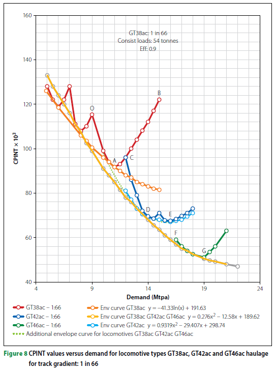
The following observations concerning the graphic plot of CPINT results were made:

■ The results formed a series of "strings" of parabolic shape, of which the lowest value represented the "vertex" of the envelope curve. Each "string", or parabolic curve, represented the application of a locomotive and a wagon consist configuration and the hauling capacity expressed in terms of the payload of the conveying unit.

■ On the range of the downward slope (O-A, C-D and F-G) of the CPINT curve the volumes were increased due to the increase in conveyance effort created by the increased number of trains (Prince 2015). The maximum efficient operating capacity was represented by the ordinates of the vertex of the curves (A, D, E and G).

■ On the range of the upward slope of a curve (A-B), dis-economies of scale were experienced due to increasing train speeds, the resultant variability and randomness occurring in train operations, and the exceedance of the in-built buffer transit times.

■ At the vertex points (A, D, E and G), the axle load could either be increased, or the train consist be supplemented to create additional haulage capacity. The shape of the envelope curve resembled the Harris curve for railway costs versus track density (Harris 1977; De Bod & Havenga 2010).

The CPINT values decreased from a demand of 5 Mtpa to 13 Mtpa for a maximum train consist of 7 locomotives and 84 wagons. This was due to the diluting of fixed costs and capacity utilisation on the mainline, exhausting the "economy of scale".

The train operations capacity was restricted to 8 trains per day in the utilisation of train crossing capacity. If the consist capacity of 7 locomotives and 120 wagons was reached (at C), the traction power was increased by deploying a more powerful type of locomotive to operate within the train crossing restrictive capacity. Consequently, the wagon consists were extended, and the axle loads increased (at C) instead of running additional light axleloaded trains to meet the demand (Boysen 2012b).

The result was that the CPINT ordinates for the GT38ac, GT42ac and GT46ac traction scenarios reduced versus increases in demand due to the deployment of additional capacity in terms of haulage power (red, blue and green curves), train consist and train-crossing capacity in terms of crossing-loop configuration.

 

CONCLUSIONS

The main objective was attained by compiling a design model that integrated the design processes of capacity creation of production factors influenced by systemic operating efficiency. The sub-objectives in this research study were also achieved, namely:

■ Sub-objective 1 was met by establishing a sub-model to determine the interrelationship between the macro geometric layout of the linear track structure and earthworks volumes.

■ Regarding the attainment of sub-objective 2, the correlation of the haulage performance of the rolling stock related to the macro geometric track alignment and the demand, was met. In this regard, a sub-model was compiled that relates the track gradients to the performance of train consists.

■ In pursuing sub-objective 3, the effect of total systemic efficiency levels on the rolling stock's capacity was determined. Simulation results informed the definition of parameters applied in the haulage sub-model. The systemic operating efficiency was deduced from scenarios of inefficient performance of train operations and the impact thereof on capacity creation and interrelated internal rate of return (IRR) quantified.

■ Sub-objective 4 was met in terms of structuring a design model that integrated the capacities and processes of a railway system. The impact of levels of inefficient operating on the IRR was derived from the financial results of the design model. The design model was developed to integrate and optimise the production factors and to determine the financial viability of a dedicated rail freight project.

The conclusion is drawn that a reduction in total systemic efficiency results in the increase of the capacity of production factors, i.e. rolling stock fleet size and, consequently, the capex and opex, which results in the escalation of the tariff rate or reduction of the IRR of a railway venture.

 

REFERENCES

Abril, M, Barber, F, Ingolotti, L, Salido, M, Tormos, P & Lova, A 2007. Assessment of railway capacity. Transportation Research PartE, 44: 774-806. https://ideas.repec.org/a/eee/transe/v44y2008i5p774-806.html.         [ Links ]

Aikaterini, K 2010. A note on the theory of productive efficiency and stochastic frontier models. European Research Studies, XIII(4): 109-118.         [ Links ]

Ball, P 2016. The Scheffel bogie and the rail gauge. The Heritage Portal. https://www.theheritageportal.co.za/article/scheffel-bogie-and-rail-gauge.         [ Links ]

BCampus Open Publishing 2019. The structure of costs in the long run. Cost and industry structure. Chapter 7.3. https://opentextbc.ca/principlesofeconomics/chapter7-3-the-structure-of-costs-in-the-long-run.         [ Links ]

Boysen, H 2012a. General model of railway transport capacity. WIT Transactions on the Built Environment (Sweden), 127(13): 335-347. https://www.researchgate.net/publication/311616164.         [ Links ]

Boysen, H 2012b. More efficient freight transport through longer trains. Transport Forum, Linkoping, Sweden. https://www.slideshare.net/hansboysen/session-42-hans-boysen.         [ Links ]

Bureika, G 2008. A mathematical model of train continuous motion uphill. Report. Department of Railway Transport, Vilnius, Lithuania.         [ Links ]

Carr, S 2016. Ask the editor: How to use effective and efficient. https://www.learnersdictionary.com/qa/How-to-Use-Effective-and-Efficient.         [ Links ]

Coals to Newcastle 2017. The application of the Davis formula to set default train resistance in open rails. Elvas Tower. https://www.elvastower.com/forums/index.php?app=core6module=attach6section=attach6attach_id=82501.         [ Links ]

Chen, C 2007 Cost functions, principles of macro-economics. Open Course. Course materials for 14.01. Lecture 13: Oxford Economic Papers, 28: 447-460.         [ Links ]

Cormen, T H, Leiserson, C E, Rivest, R L & Stein, C 1990. Introduction to Algorithms, 2nd ed. Cambridge, MA: MIT Press & McGraw-Hill.         [ Links ]

Davis, W 1926. Tractive resistance of electric locomotives and cars. General Electric Review, 29: 685-708.         [ Links ]

De Bod, A & Havenga, J 2010. Sub-Saharan Africa's rail freight transport system: Potential impact of densification costs. Journal of Transport and Supply Chain Management, 4(1). https://doi.org/10.4102/jtscm.v4i1.13.         [ Links ]

Denley, M 2018. Research into enhanced tracks, switches and structures. IN2TRACK Shift2Rail Innovation Programme 3. European Union. Brochure No. GA H2020 730841. https://www.projects.shift2rail.org.         [ Links ]

Dhali, M N, Bulbul, M F & Sadiya, U 2019. Comparison on trapezoidal and Simpsons rule for unequal data space. International Journal of Mathematical Sciences and Computing, 4: 33-43. http://www.mecs-press.net/ijmsc.         [ Links ]

Drury, C 2009. Management Accountingfor Business, 4th ed. Singapore: Seng Lee Press.         [ Links ]

Duffy, D P 2018. Estimating earthwork volumes. GX Contractor. https://www.gxcontractor.com/technology/article/13034514/estimating-earthwork-volumes.         [ Links ]

Dutton, C J & Mülke, F J 2017. Systemic railway engineering relevance in heavy haul railway systems. Proceedings, 11th International Heavy Haul Association Conference, 2-6 September 2017, Cape Town. https://ihha.net/resources-ihha/2017-conference-proceedings.         [ Links ]

Esveld, C 1989. Modern Railway Track. Chapter 10. Duisberg, Germany: MRT-Productions, pp 249-259.         [ Links ]

Ghoreishi, B H 2019. A model for optimising railway alignment considering bridge costs, tunnel costs and transition curves. Urban Rail Transit, 5: 207-224.         [ Links ]

Grosskopf, S 1993. Efficiency and productivity. Chapter 4. In Fried, H O (Ed). The Measurement of Productive Efficiency: Techniques, and Applications. New York: Oxford University Press, pp 160-194.         [ Links ]

Harris, R 1977. Economies of traffic density in the rail freight industry. The Bell Journal of Economics, 8(2): 556-564.         [ Links ]

Indian Railways Institute. n.d. Horsepower and design parameters. http://www.irimee.indianrailways.gov.in/instt/uploads/files/1477552393969-Horsepower_6_Design_Parameters_of_GM_Locomotive.pdf.         [ Links ]

Jondrow, J 1982. On the estimation of technical efficiency in the stochastic frontier production function model. Journal of Econometrics, 19: 233-238.         [ Links ]

Kay, J A 1976. Accountants, too, could be happy in a Golden Age: The accountant's rate of profit and the internal rate of return. Oxford Economic Papers, 28(3): 447-460.         [ Links ]

Krueger, H 1999. Parametric modelling in rail capacity planning. Proceedings, 1999 Winter Simulation Conference, Montreal, Quebec, Canada.         [ Links ]

Kuys, W, Fenske, A & Klahn, V 2017. Exploring the advantages of operating a scheduled railway in the South African context. Proceedings, 11th International Heavy Haul Association Conference, 2-6 Sept 2017, Cape Town. https://ihha.net>resources.Ihha>2017-conference-pro.         [ Links ]

Kweon, I S & Kanade, T 1994. Extracting topographic terrain features from elevation maps. CVGIP: Image Understanding, 59(2): 171-182.         [ Links ]

Leonard, J 1986. A strategic investment decision model for line haul operations on a developing country railway. PhD Thesis. UK: University of Leeds.         [ Links ]

Lindfeldt, A 2015. Railway capacity analysis: Methods for simulation and evaluation of timetables, delays and infrastructure. Report. Stockholm, Sweden: KTH Royal Institute of Technology, Department of Transport Science. ORCID ID: 0000-0002-5192-8074.         [ Links ]

Lombard, P C 1976. Trackwork structure: Relationship between structure parameters, traffic volumes and maintenance. MSc Dissertation. University of Pretoria.         [ Links ]

Lombard, P C 2017. Composing a heavy haul engineering symphony in differential life cycle costing. Proceedings, 11th International Heavy Haul Association Conference (IHHA 2017), 2-6 September 2017, Cape Town. https://ihha.net/resources-ihha/2017-conference-proceedings.         [ Links ]

Lozano, J A, Felez, J, De Dios Sanz, J & Mera, J M 2019. Hauling power of a locomotive. https://eng.dieselloc.ru/railway-engineering/hauling-power-of-a-locomotive.html.         [ Links ]

Luiu, C, Torbaghan, M & Burrow, M 2018. Rates of return of railway infrastructure investments in Africa. Birmingham, UK: University of Birmingham. https://www.researchgate.net/publication/330204040.         [ Links ]

Mallery, T 2010. Tractive force and hauling power. Catskill Archive. https://www.catskillarchive.com/articles.htm.         [ Links ]

McGonigal, R 2006. Grades and curves. Trains Magazine. https://trn.trains.com/railroads/abcs-of-railroading/2006/05/grades-and-curves.         [ Links ]

Mülke, F J, Havenga, J H & Van Eeden, J 2021. Systemic efficiency: A key consideration in the design of dedicated rail freight projects in southern Africa. South African Journal of Industrial Engineering, 32(3): 211-224. https://doi.org/10.7166/32-3-2635.         [ Links ]

Parajuli, A 2005. Modelling road and rail freight energy consumption: A comparative study. MEng Dissertation. Queensland University, Australia.         [ Links ]

Pettinger, T 2019. Diagrams of cost curves. (Blog). http://economicshelp.org/blog/189/economics/diagrams-of-cost_curves.         [ Links ]

Preston, J 1992. A simple model of rail infrastructure capacity and costs. Working Paper No 370. Leeds, UK: University of Leeds, Institute of Transport Studies.         [ Links ]

Prince, A 2015. Capacity factors in intermodal road-rail terminals. MSc Thesis. Gothenburg, Sweden, University of Technology. https://publications.lib.chalmers.se/records/fulltext/224972/224972.pdf.         [ Links ]

Rauch, H (Chief Geotechnical Engineer, SAR&H). n.d. Personal discussions.         [ Links ]

Riley, S J, De Gloria, S D & Elliot, R 1999. A terrain ruggedness index that quantifies topographic heterogeneity. Intermountain Journal of Sciences, 5(1-4): 23-27. https://download.osgeo.org/qgis/doc/reference-docs/Terrain_Ruggedness_Index.pdf.         [ Links ]

Roney, M 2015. The fundamentals of vehicle/track interaction. In: Guidelines to Best Practices for Heavy Haul Railway Operations. International Heavy Haul Association (IHHA). Virginia Beach, VA, pp 2-65.         [ Links ]

Sameni, M 2012. Railway track capacity: measuring and managing. South Hampton, UK: University of South Hampton.         [ Links ]

Samuelson, P 1970. Economics. New York: McGraw-Hill.         [ Links ]

SAR&H (South African Railways and Harbours) 1968. The Green Book. Johannesburg: SAR&H.         [ Links ]

Scheffel, H & Von Gericke, R 1983. The development and design of the Scheffel self-steering truck and in-service experience gained on the South African Transport Services (SATS). Johannesburg: SATS.         [ Links ]

Skempton, A 1996. Embankments and cuttings on the early railways. Construction History, 11: 33-49.         [ Links ]

Szanto, F 2016. Rolling resistance revisited. Proceedings, Conference on Railway Excellence, 16-18 May 2016, Melbourne, Australia. https://www.scribd.com/document/423130043/Szanto-Frank.         [ Links ]

The Mathematical Association (UK) 2004. Tractive effort, acceleration and braking. Transport: Railways. https://www.m-a.org.uk/what_use/TractiveEffortAccelerationAndBraking.doc.         [ Links ]

Tourney, H & Fröhling, R 2015. Rail and wheel mechanics. Chapter 3. In: Guidelines to Best Practices for Heavy Haul Operations. International Heavy Haul Association (IHHA). Virginia Beach, VA: Simmons-Boardman Books, pp 3-1 - 3-28.         [ Links ]

UIC (International Union of Railways) 2015. Appendix 11: Long List of Cost Drivers. Paris, France: UIC Asset Management Working Group.         [ Links ]

Zuan, X 2007. Train dynamics. MEng Dissertation. University of Pretoria.         [ Links ]

 

 

Correspondence:
F J Mülke
Department of Industrial Engineering, Stellenbosch University
Private Bag X1, Matieland 7602, Stellenbosch, South Africa
E: mulke@netactice.co.za

J H Havenga
Department of Industrial Engineering, Stellenbosch University
Private Bag X1, Matieland 7602, Stellenbosch, South Africa
E: janh@sun.ac.za

J van Eeden
Department of Industrial Engineering, Stellenbosch University
Private Bag X1, Matieland 7602, Stellenbosch, South Africa
E: jveeden@sun.ac.za

 

 

 

DR FRIEDEL MÜLKE (Pr Eng, FSAICE, MSAIIE) joined the Construction Department of the erstwhile SAR&H (South African Railways and Harbours) in 1972 and spent eight years on new railway line construction projects. Following an operations career in managerial positions with the South African Transport Services and Transnetforthe next 19 years, he changed course to become a consultant in railway projects. For the next 24 years, he served as project manager, operating lead, and railway specialist in developing various new dedicated rail freight projects in Southern and East Africa. In addition to his degrees in Civil Engineering, he also obtained a DEng degree from the University of Pretoria in 1981, and an MBL from the University of South Africa in 1985. He is currently a PhD candidate in Industrial Engineering at Stellenbosch University.

 

 

PROF JAN HAVENGA is an Emeritus Professor in the Department of Industrial Engineering at Stellenbosch University. He is a pioneer in the emerging field of macrologistics. This field applies the principles of business logistics in national and international contexts through freight-flow research to inform sustainability, policy development and infrastructure investments. He has led a large number of national and regional projects in this regard throughout Africa and Asia. Currently he is a member of the Operation Vulindlela team in the office of the President that was tasked to coordinate a roadmap for a turnaround of South Africa's logistics system.

 

 

PROF JOUBERT VAN EEDEN is an Associate Professor and Chair of the Department of Industrial Engineering at Stellenbosch University. He obtained a PhD in Industrial Engineering and an MBA through Stellenbosch University, where he now lectures in Supply Chain Management. He developed the Container Demand Model used by Transnet Group Planning to inform port and rail infrastructure planning in terms of national port and domestic container volumes. He has an interest in macrologistics modelling, and conducts research within logistics management and sustainable freight transport. He furthermore provides research guidance to graduate students in the fields of Supply Chain and Logistics Management, and Freight Modelling.