GENERAL ARTICLES

 

Inventory Management using Reinforcement Learning

 

 

B.I. Smith; A. Garg; W.B.A. Rich

School of Mechanical, Industrial and Aeronautical Engineering, University of the Witwatersrand, Johannesburg, South Africa

 

 

---

ABSTRACT

Poor inventory management negatively affects a company's profits. Too little stock limits potential sales and customer satisfaction, while too much stock increases storage costs and potential damage. This study combined supervised and deep reinforcement learning (DRL) for optimal decision-making that would maximise profits in the supply chain of Company X. The performance was compared with a benchmark heuristic that stocks inventory based on a seven-day forecast. The DRL models achieved a marginally lower net profit, but satisfied significantly lower customer demand compared with the benchmark heuristic, thus showing its potential to help to optimise the supply chain structure, operation, and parameters.

---

OPSOMMING

Swak voorraadbestuur het 'n negatiewe invloed op 'n maatskappy se wins. Te min voorraad beperk potensiële verkope en kliëntetevredenheid, terwyl te veel voorraad bergingskoste en potensiële skade verhoog. Hierdie studie het toesig- en diep versterkingsleer (DRL) gekombineer vir optimale besluitneming wat wins in die voorsieningsketting van Maatskappy X sou maksimeer. Die prestasie is vergelyk met 'n maatstafheuristiek wat voorraad op grond van 'n sewe-dae voorspelling in voorraad hou. Die DRL-modelle het 'n marginaal laer netto wins behaal, maar het aansienlik laer kliënte-vraag bevredig in vergelyking met die maatstafheuristiek, en toon dus die potensiaal daarvan om te help om die voorsieningskettingstruktuur, -werking en -parameters te optimeer.

---

 

 

1. INTRODUCTION

Inventory management involves planning, manufacturing, and distributing goods to maintain optimal stock levels, meet customer demand, and maximise profits. Supply chains - that is, sequential networks of processes - store inventory to manage demand fluctuations and to benefit from economies of scale [1]. Poor management, including inaccurate demand forecasting, can lead to the bullwhip effect, in which small fluctuations in customer demand at the retail level cause progressively larger variations in demand and inventory levels as one moves up the supply chain [2]. Overstocking increases costs, while understocking leads to lost sales. Traditional inventory management methods, such as economic order quantity (EOQ) or reorder point models, often assume stable demand and consistent lead times. These methods may struggle to account for stochastic constraints such as demand variability, especially in complex, dynamic supply chains [3]. This is why advanced techniques such as machine learning (ML) or reinforcement learning (RL) are increasingly used to manage variability and uncertainties in modern supply chains [4].

This research investigated the use of reinforcement learning to improve inventory management for Company X, a butter producer and distributor, using real company data. Key points about Company X's supply chain were the following:

- Reducing storage costs by around 5% could save just under R1m annually.

- The fill rate (percentage of customer demand met) is 95%. Not meeting 1% of demand results in a yearly revenue loss of over R18 million.

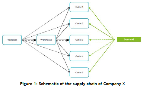
The supply chain of Company X includes a production unit, a warehouse, and five outlets (see Figure 1). Key supply chain data such as demand, costs, capacities, and lead times were analysed to find the best production, distribution, and storage strategies to maximise profits. Company X currently uses a heuristic (a practical strategy to make quick decisions) to store inventory, based on forecast demand: seven days for outlets and twelve days for the warehouse. This guides stock replenishment to maximise profits. Machine learning (ML) could improve this by incorporating the supply chain's variability to determine optimal order quantities at each time step.

 

 

This study sought to investigate how reinforcement learning (RL) compares with heuristic techniques in respect of net profit. The main contributions of this work are:

- Reinforcement learning (RL) was applied to a real case using a unique combination of real supply chain parameters and unique action, state, and reward variables. This benefits the inventory management community by showing how to model a more complex supply chain using real supply chain data from a company (Section 1 ).

- A combination of supervised learning and reinforcement learning was applied to an inventory management system. Supervised learning was applied to forecast the demand, which fed into the training of a reinforcement learning model (Section 3).

- RL helps determine which aspects of a supply chain are working well. It showed the potential of advising certain business decisions in the future relating to supply chain structure, pricing, and distribution of goods, based on current trends (Section 4.4).

- To the best of our knowledge, this is the first research that has applied the deep deterministic policy gradient (DDPG) algorithm to a multi-echelon inventory system with a general network structure (stock points having many successors and many predecessors), using real supply chain data. The DDPG model achieved a marginally lower net profit, but it satisfied demand from about half the outlets in the supply chain compared with the benchmark heuristic (Section 4.5).

 

2. LITERATURE REVIEW

This section reviews the literature on the machine learning models used in this study (both supervised and reinforcement learning) and on applying RL to inventory management.

2.1. Supervised learning

Supervised learning was used to forecast demand. Supervised learning was not the primary focus of this study, and therefore we do not discuss it in detail. Four regression models, namely linear regression, K-nearest neighbours (KNN), random forest (RF), and support vector machine (SVM), were trained on the historic daily demand data. These models are summarised below:

- Linear regression is a fundamental model that establishes a relationship between independent variables and a continuous dependent variable by fitting a straight line (hyperplane in higher dimensions). The model minimises the sum of squared residuals between observed and predicted values [5].

- K-nearest neighbours (KNN) is a non-parametric model that predicts the target value, based on the average of the k nearest data points (neighbours) in the feature space. It relies on distance metrics, typically Euclidean, and can capture local patterns, but is sensitive to outliers and data scaling [6].

- Random forest is a powerful ensemble model that builds multiple decision trees during training and aggregates their predictions for more robust and accurate outcomes. By using bootstrap aggregation and random feature selection, it reduces overfitting and improves generalisation [7].

- Support vector machines (SVM) regression (SVR) aims to fit a model within a specified error margin (epsilon) by constructing hyperplanes that maximise the margins between data points. It is effective for high-dimensional data, but can be computationally expensive for large datasets [8].

2.2. Reinforcement learning

The forecast demand from the supervised regression models forms an input to the heuristic and RL models, which aim to determine an optimal ordering strategy that maximises profits in the supply chain. This input was incorporated into the RL feedback loop, as shown in Figure 2 [9]. RL involves an agent making decisions in an environment to maximise a goal. Depending on the current state S_t of the environment, the agent selects a particular action A_t, receives feedback in the form of a reward R_t+1, and transitions to a new state S_t+1 in the environment [9]. The agent trains through many iterations, using rewards that indicate how good or bad the actions are in each state.

 

 

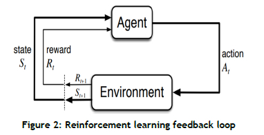
In RL, the Markov property states that the future state depends only on the current state and action, not on prior events. A Markov decision process (MDP) models decision-making such that outcomes are both controlled and random, using components such as states, actions, rewards, and policies [9]. This section explains key RL terminology, while the next covers RL algorithms.

2.2.1. Agent

The agent (or algorithm) is the decision-making entity that learns a strategy to achieve a specific goal in an environment. The agent could represent a supply chain manager overseeing the entire supply chain [10].

2.2.2. Environment

The environment is the external structure with which an RL agent interacts [10]. It contains the agent, action space, state space, and rewards to achieve a particular goal. For this research, a custom inventory management environment was developed.

2.2.3. Action space

The action space includes all possible actions the agent could take, such as ordering quantities in a supply chain. Actions can be discrete, with fixed order amounts, or continuous, allowing agents to adjust ordering or production rates within a range [10]. A continuous action space is preferred for this application, as it enables agents to adapt actions to specific conditions, optimising profitability.

2.2.4. State/observation space

A state is a partial or full description of the environment in which the agent is operating at a particular point in time. It needs to be carefully defined to provide an efficient decision-making process for the agent [10]. It can include any combination of the supply chain variables and parameters that are used.

2.2.5. Rewards

RL models are trained by maximising a long-term reward. Rewards are therefore vital for training RL models, as they guide the RL model in achieving its objective, such as maximising profits or minimising loss [10]. In inventory management, reward functions may consider factors such as current profit per time step, fill rate, and available units. Return is the cumulative reward received by the agent over an episode, summarised by Equation 1, where R, is the return; t, is the specific time step in the episode; N, is the termination time step; is the reward at time step t; and y, is the discount factor that determines the importance of future rewards.

2.2.6. Time steps and episodes

RL models learn using a trial and error process in which each time step represents one increment of the agent taking an action in a given state and receiving a reward to reach a new state [10]. An episode is one iteration of the agent, starting from an initial state in the environment, such as starting at day 0, until it reaches a terminal state in the environment, such as reaching a period of a year.

2.2.7. Exploration and exploitation

At each time step, the agent either explores or exploits the environment. Exploring involves selecting an action randomly to try new actions that may lead to better outcomes in the future. Exploitation involves selecting the best action, based on current information and past experiences. An epsilon-greedy approach is commonly used to balance the trade-off between exploration and exploitation, using an exploration rate e [11]. This parameter has a value between 0 and 1, with a higher value encouraging exploration.

2.2.8. Policy

Ultimately, the RL agent needs to learn a policy, which is a mapping of states to actions [10]. That is, if an agent observes a state, what is the best action to take to maximise a long-term reward?

2.2.9. Value-based learning and policy-based learning

Essentially, two approaches are used in reinforcement learning (RL) to train an agent to learn an optimal policy: value-based learning and policy-based learning.

In value-based methods, the goal is to estimate how good it is to be in a particular state, either through a state-value function V(s) or a state-action value function Q(s,a). V(s), the state-value function, indicates how valuable it is to be in that state; and the agent uses this information to select actions that lead to states with higher values [10]. Q(s,a), the action-value function, indicates the value of being in a state and taking a specific action [12]. This approach tells the agent directly how valuable it would be to take a specific action in a given state, allowing it to choose actions based on their Q-values. It focuses on state-action pairs.

With value-based methods, we first calculate the value in each state. The optimal policy is then obtained by taking a further step to identify the best actions. Policy-based learning, however, bypasses this step, and optimises directly for the policy by mapping states to actions to maximise a long-term reward [12].

Proximal policy optimisation (PPO) is one of the most common policy optimisation algorithms. Deep deterministic policy optimisation (DDPG) is a popular algorithm that combines both Q-learning and policy optimisation. These models were used in this study. We discuss them next.

2.2.10. Proximal policy optimisation

PPO is a method that combines both policy- and value-based methods in the form of an actor (policy) that decides which action to take in each state, and a critic (value) that estimates how good each action was by estimating the state-value function V(s). The actor and critic are deep learning neural networks [13]. An important component of PPO is a quantity called 'advantage' that estimates how much better (or worse) an action is than the expected value of being in a particular state. We then reinforce the actions that produced positive advantage, and discourage actions that produced negative advantage. Mathematically, the advantage A(s,a) is defined as:

Q(s,a) is the expected reward for taking action a in state s.

V(s) is the expected reward for just being in state s.

2.2.11. Deep deterministic policy gradient (DDPG)

Deep deterministic policy gradient (DDPG) is a reinforcement learning algorithm that operates in continuous action spaces using an actor-critic architecture that is similar to PPO [14]. The actor outputs deterministic actions (rather than a probability distribution) for a given state, which makes DDPG well-suited for problems with continuous actions, such as robotic control. The critic helps to guide the actor's updates by providing feedback on the quality of the selected actions. An essential aspect of DDPG is its use of experience replay and target networks. Experience replay stores past interactions (state, action, reward, next state) in a buffer, and samples mini-batches of data for training, which reduces correlations between samples and stabilises learning.

2.3. Traditional inventory control methods

Just-in-time (JIT) management orders goods as needed, reducing inventory costs but posing risks if demand spikes or delays occur [3]. Reorder point (ROP) management triggers orders when stock reaches a minimum level, preventing stockouts but failing to optimise inventory turnover or order quantities. Days sales of inventory (DSI) shows average inventory days, but does not account for product value or supply chain factors. The economic order quantity (EOQ) model assumes constant demand and complete information, which is unrealistic in real supply chains with fluctuating demand and uncertainty. Reinforcement learning (RL), however, can adapt ordering strategies more effectively, based on current inventory conditions.

2.4. Machine learning applications in supply chains

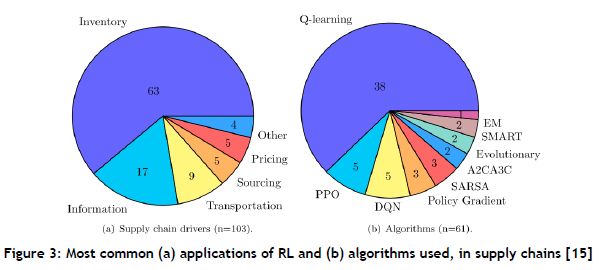
Figure 3 shows that 63% of RL models that are applied to supply chains focus on inventory management. It also shows that Q-learning is the most common algorithm owing to its model-free nature, which allows agents to sample and learn from expected rewards without needing an environment model [15].

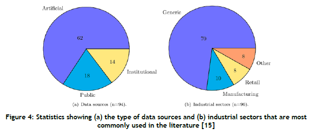
Useful supply chain data for designing RL agents includes network structure, lead times, forecast demand, suppliers, costs, and constraints. Figure 4 shows that artificial data is most commonly used because of the limited availability of real data. Using real data can improve RL models by making them more applicable to real-world scenarios. Most research uses generic settings with simple supply chains, low uncertainty, and few constraints. Although manufacturing and retail supply chains are often considered, research in these sectors remains limited [15].

Deep reinforcement learning (DRL) has been applied to multi-echelon supply chains, optimising inventory levels across all stock points. State variables represent inventory position, actions represent order quantity, and rewards are based on profit. Gijsbrechts et al. used the A3C algorithm, achieving a 9% improvement over the base stock policy [16]. Hubbs et al. [17] and Xie et al. [18] applied PPO, improving performance over traditional policies by 11% and 18% respectively. Oroojlooyjadid et al. [19] used DQN and achieved a 13% cost reduction, while Geevers et al. [20] applied PPO but experienced instability, with actions correct only 50% of the time. However, the best simulations reduced costs by 20%. Both last-named tudies used multi-agent approaches to optimise stock points under capacity constraints.

 

3. METHOD

Most literature sources use many assumptions and simplifications, such as artificial demand datasets, constant lead times, and limited stock points (simple/linear supply chain network), and do not include their code, which makes them less reproducible. This research considered the real supply chain data of a butter company to predict the forecast demand, which was used as input to an RL model. A single product (butter) was considered in this research simultaneously to minimise costs and to maximise profits and the fill rate. A finite time horizon, continuous action space, and a single-agent analysis were used, thus streamlining the RL model (fewer variables and dependencies). A custom RL environment, using unique state, action, and reward variables, was created together with DRL algorithms (PPO and DDPG) to train an agent more effectively than existing RL environments do; this was done in an attempt to improve the inventory management of the company. This research involved using an online RL model, since the agent directly interacts with the environment to reach new states. One full year constituted an episode, after which the model was reset to the original starting state.

The following methodology was used:

- Use supervised learning to perform demand forecasting by learning the trends and features of the historical sales dataset. The demand forecasts provide useful input data to both the heuristic and the RL models in order to help plan inventory ahead of time.

- Incorporate the company heuristic into the supply chain workflow to obtain a baseline inventory management model.

- Develop a custom RL environment and train PPO and DDPG algorithms to plan, track, and optimise inventory in the supply chain to maximise profits.

3.1. Modelling the particular supply chain

The production facility produces a certain number of units between the minimum and maximum production limit while considering its storage capacity and the production processing time before the units become finished inventory. The warehouse orders a certain number of units from the production facility, and the outlets order a certain number from either the warehouse or the production facility. The order quantity considers the units available at the upstream location, the storage capacity of the warehouse/outlet, the truck capacity, and the transport time between the respective facilities. The orders placed from a stock point to an upstream facility are placed in a backlog variable, as units can only be sent when the upstream facility has sufficient units available. Revenue is gained by fulfilling customer demand at the warehouse and at each outlet. The first in, first out (FIFO) inventory method is applied to reduce the chances of obsolete inventory occurring. The overall cost, including manufacture, delivery, and storage costs, is calculated; and finally the overall net profit and fill rate are calculated.

- Various assumptions about this particular supply chain were made:

- Unlimited raw material supply;

- A fixed sales price;

- Single butter product type;

- Perpetual inventory control (fast-moving consumer goods [FMCG] style);

- Backorders not considered;

- Quality is maintained.

3.2. Benchmark heuristic for inventory management

We developed a heuristic model as follows: the number of units ordered upstream for each outlet was based on seven days of their respective forecast demand, while the warehouse was based on its twelve-day forecast demand. This replicated the approach used in the company. The initial units available at each of the outlets and the warehouse on day 1 to begin the simulation were based on the same idea.

3.3. Reinforcement learning for inventory management

The OpenAI Gym structure was used to create a custom RL environment that incorporated the supply chain workflow with the same conditions as those in the heuristic to allow both methods to be compared [21].

3.3.1. Action space

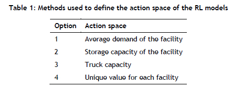
At every time step, an ordering quantity (action) is placed from the warehouse and from each of the outlets to an upstream facility in the supply chain, and production decides on a certain number of units to produce (action). A random choice was used to determine whether the outlets ordered from the production facility or from the warehouse. A continuous action space was used that output a normalised value between 0 and 1. It therefore needed to be scaled up to represent a realistic ordering quantity. Different methods based on the average demand, storage capacity, truck capacity, or unique optimisation could be used to determine the scaling factor for the warehouse and for each outlet, as summarised in Table 1.

 

 

3.3.2. State space

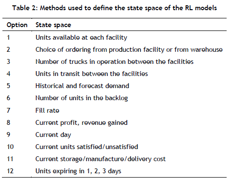
Table 2 shows various state space parameters. Various combinations of these were used to determine which combination would provide the highest net profit.

 

 

3.3.3. Reward function

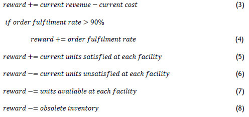
Different methods were used to develop and test the reward function, including profit per time step (Equation 3), fill rate (Equation 4), maximising the number of units sold (Equation 5), minimising unsatisfied demand (Equation 6), minimising number of units available (Equation 7), and minimising obsolete inventory (Equation 8). Reward shaping was applied by including scaling factors in each reward to give priority to certain scenarios. Different combinations of these reward functions with unique reward shaping were tested to find the best reward function that provided the highest net profit for this research.

Extremely large values in the state space and reward function can lead to unstable and unpredictable behaviour, making it difficult for the agent to learn and generalise to new states in the environment. Thus, the variables used in the state space and the reward function are normalised using min-max normalisation into a fixed range. The hyperparameters of the PPO and DDPG algorithms used in this research were tuned in an attempt to improve the performance of the RL model.

 

4. RESULTS AND DISCUSSION

4.1. Demand forecast from supervised learning

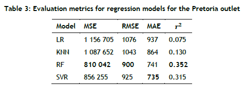
The first step was to train supervised regression models to predict the demand forecast, which would serve as an input into the heuristic and RL models. Random forest performed the best by achieving the lowest error and highest correlation, as shown in Table 3; thus it was subsequently used.

 

 

4.2. Benchmark heuristic

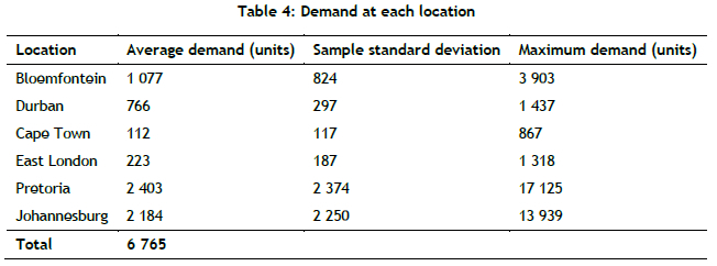
The original minimum production limit of 30,000 units per day caused the production facility to reach its storage capacity quickly, leading to increased storage costs and obsolete inventory. This mismatch between supply and demand significantly reduced net profits, as the average demand across all locations was only 6,765 units (see Table 4). A value of 5,000 units for the minimum production limit provided the best performance for the heuristic model.

4.3. RL results

4.3.1. State space

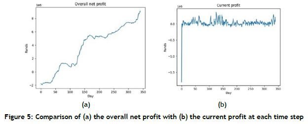
We found that using cumulative variables in the state space was ineffective, as they resulted in an infinite state space, which led to an inefficient learning process. Variables based on the current value, such as current profit as opposed to overall profit (as shown in Figure 5), were more effective.

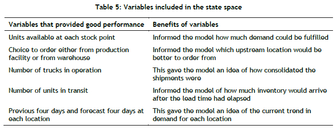
Table 5 shows the variables that were found to be useful to include in the state space.

4.3.2. Reward function

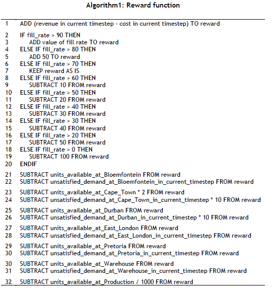
Maximising a positive reward by adding the current units that were satisfied to the reward did not provide any performance improvement. However, subtracting the current units that were unsatisfied provided improved performance. Thus, it was concluded that it was better to minimise a negative reward in the RL model for this application.

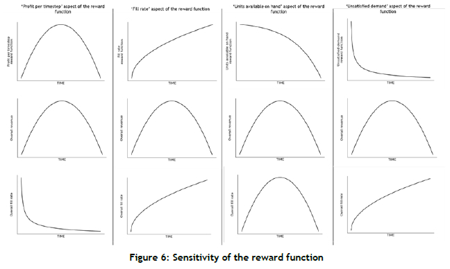
The general trends showing reward function sensitivity for different considerations in the reward function over the period of a single episode are shown in Figure 6. For the 'profit per time step' aspect of the reward function, the model showed that the reward increased initially, reached a peak, and then decreased. The overall revenue followed a similar trend, while the overall fill rate quickly decreased in a hyperbolic fashion. For the 'fill rate' aspect of the reward function, both the reward and the overall fill rate increased to a smaller extent over time, while the overall revenue followed an upside-down parabolic trend. For the 'units available on hand' aspect of the reward function, the reward decreased to a larger extent over time, while the overall revenue and fill rate followed an upside-down parabolic trend. For the 'unsatisfied demand' aspect of the reward function, the reward decreased quickly in a hyperbolic fashion, and the overall revenue followed an upside-down parabolic trend, while the fill rate increased to a smaller extent over time.

Multiple combinations were tested, but a reward function based on a combination of profit per time step, fill rate, units available on hand, and units unsatisfied provided the highest net profit at the end of the year. We also found that using a constant reward value for a particular range of states was not always effective, as static conditions could become highly non-linear. Thus, unique scaling factors (reward shaping) were used in the reward function to indicate that certain scenarios were better than others. This proved to be effective in improving the net profit of the RL model. However, the reward function was highly sensitive, and it had a significant effect on the performance of the RL models. The final reward function is shown in pseudocode below.

 

 

4.3.3. Action space

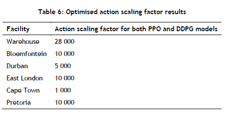
Scaling up of the action space was tested using the storage/truck capacity and a factor of the average demand at each location. Using a factor of the storage/truck capacity provided a higher fill rate but achieved a lower net profit when compared to using a factor of the average demand. The RL agent learns to send consolidated trucks most of the time to save on costs. Large amounts of time are required before upstream locations store sufficient goods to send full trucks, thereby reducing the fill rate. Possible solutions included increasing the starting inventory, increasing the minimum production limit, altering the reward function and using a unique scale-up of the action space for each location. After iterating through multiple scale-up factors, the quantities in Table 6 for each location provided the best performance.

 

 

4.3.4. Hyperparameters

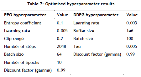
Hyperparameter tuning was performed using the random search method, in which hyperparameters were randomly sampled from a defined distribution. The final hyperparameter values for the PPO and DDPG models are presented in Table 7. The entropy coefficient of PPO and the learning rate and discount factor of both PPO and DDPG were the most sensitive to the model's performance. These values were found to provide the best balance between model exploration and exploitation.

 

 

4.3.5. Comparing the heuristic and RL models' results

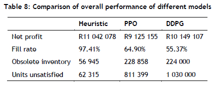
Table 8 shows that, for the heuristic model, significantly fewer units were unsatisfied or obsolete inventory, resulting in a higher fill rate than with the PPO and DDPG models. Both the PPO and the DDPG models achieved a marginally lower net profit, but at a significantly lower fill rate. A lower inventory investment resulting in a lower fill rate led to less profit because of insufficient inventory. Similarly, a higher inventory investment resulting in a higher fill rate also led to less profit, but this was due to excess inventory increasing holding costs. This indicated that the optimal condition was reached and that a higher fill rate in a supply chain would not necessarily lead to a higher net profit. The extremely high number of unsatisfied units in the PPO and DDPG models limited their profitability; surprisingly, however, they still achieved a net profit that was relatively close to the heuristic model. Although not performing well here, the PPO and DDPG models could help to optimise the supply chain structure, operation, and parameters in the future, possibly increasing the net profit beyond that of the heuristic.

 

 

The RL models provided useful insights such as these:

- Shipment consolidation was preferred, as delivery costs exceeded storage costs.

- No orders were placed by the DDPG model at the Durban, East London, or Cape Town outlets owing to higher delivery costs: these three locations were the furthest from both the production facility and the warehouse. In addition, these three locations had the lowest average demand across the year. Thus, the model may have learnt that the inventory investment in sending units to these locations exceeded the revenue obtained from satisfying customer demand.

- The RL models learnt that sending units directly from the production unit to the outlets was cheaper and quicker while sending only a small amount of surplus stock to the warehouse for storage.

4.4. Comparison with prior work

Considerable research has been performed on inventory management using RL; yet it remains difficult to determine when and how much to order because of the curse of dimensionality (exponential increase in data and computation as the number of variables increases). Most literature sources use many assumptions and simplifications, such as artificial demand datasets, constant lead times, and limited stock points (simple/linear supply chain network), and do not include their code, which makes them less reproducible. This study focused on a real supply chain case using a unique combination of real supply chain parameters and unique action, state, and reward variables.

The research by Geevers et al. [20] aligned most closely with our research because they also used real historic demand, a multi-echelon supply chain, the PPO algorithm, and a custom RL environment. A continuous action space representing the ordering quantity was used in both studies; but the model used by Geevers et al. struggled to learn the interval of the action space effectively. The PPO model in our research learnt to order either 0 units or the maximum ordering quantity at each outlet, whereas the DDPG model learnt to order a constant amount - but only at certain outlets, in order to save on delivery costs. The RL models also struggled to vary the actions in this study, which resulted in large amounts of inventory being stored (storage costs) and obsolete inventory at various locations.

The state space in previous research papers varied, based on the amount of supply chain information that was available. The research by Geevers et al. focused solely on reducing inventory costs; thus, the holding and backorder costs were included only in the reward function. Our research aimed to maximise net profit and fill rate simultaneously in the supply chain without considering backorders. Thus, the reward function was based on a combination of profit per time step, fill rate, units available on hand, and units unsatisfied, with each contributing to improved performance. The reward function of Geevers et al. was also tested in this research, using the holding costs and the units unsatisfied instead of the backorder costs; but it was not able to provide better results in this particular supply chain. However, both studies showed that it was more useful to minimise a negative reward.

Both pieces of research incorporated the available inventory and the inventory in transit at each point in the supply chain. Geevers et al. also included the total backorders and total inventory in the supply chain, possibly because a multi-agent analysis was used. Our research was based on a single-agent analysis. It was found to be not useful to include the total inventory in the supply chain in the state space. The inclusion of the number of trucks in operation and the number of units in transit between various locations in this supply chain provided improved performance, as this helped the model to understand how best to use the trucks. Both studies showed that it was more useful to use current variables than cumulative variables in order to prevent an infinite state space.

 

5. CONCLUSION, LIMITATIONS, AND RECOMMENDATIONS

This study investigated the effectiveness of reinforcement learning (RL) in optimising inventory management for Company X compared with the company's existing heuristic approach. Using real supply chain data, we applied a combination of supervised learning for demand forecasting and reinforcement learning for dynamic decision-making.

Specifically, we implemented the DDPG and PPO algorithms in a multi-echelon inventory system with a general network structure - an approach not previously explored in the literature. The aim was for the RL models to learn optimal ordering strategies, with the DDPG algorithm outperforming PPO in maximising net profit. However, neither RL model outperformed the company's current heuristic approach, with the heuristic model achieving higher net profits. The RL models still provided valuable insights for improving inventory management, such as better transparency, asset use, and inventory turnover.

The RL models in this study faced several limitations, including insufficient inventory to meet demand because stock points were ordered in small quantities. Although training over time helped the models learn to order larger quantities, computational time was a significant bottleneck, even though multiprocessing was used to speed up the process. Another problem was the continuous action space, which required scaling up actions to realistic ordering quantities; the best results were achieved by using unique scaling for each stock point. Including current profit in the reward function also led to models ordering maximum quantities frequently, which caused delays owing to insufficient units being at upstream facilities.

The models also struggled with sensitivity to multiple parameters, making optimisation difficult. They failed to develop adaptive ordering strategies, resulting in excess and obsolete inventory at various locations. External factors such as customer perception and societal impact were not considered in the RL models, as these factors fell outside the study's scope. While the RL models performed well in short-term simulations, further investigation would be needed to assess long-term performance and integration with the company's ERP system before applying the RL models in practice. However, the models provided insights into the root causes of inefficiencies in the current supply chain operations.

Future research should focus on expanding the dataset with more historical demand data in order to improve forecasting accuracy, potentially integrating recurrent neural networks (RNNs) for better time-series predictions. Additional RL models could be tested with new products in the supply chain to evaluate their impact on profitability. The models' performance could also be enhanced by refining the reward function, testing advanced RL algorithms, and adapting techniques such as reducing the learning rate over time to improve policy learning.

Further exploration could address RL's sensitivity to supply chain sequencing by investigating synchronous operations and shuffling inventory distribution orders. Regularisation and random sampling techniques could enhance the generalisation of the models, while expanding the action space to include warehouse vs production ordering decisions might optimise efficiency. Finally, RL models could be used to simulate the effects of changes in supply chain structure, pricing, and distribution in order to provide data-driven business recommendations.

 

REFERENCES

[1] D. J. Bowersox, D. J. Closs, J. C. Bowersox and M. B. Cooper, Supply chain logistics management. New York: McGraw-Hill Education, 2020.         [ Links ]

[2] K. Ahmed, "What is bullwhip effect?" WallStreetMojo, 2022. [Online]. Available: https://www.wallstreetmojo.com/bullwhip-effect/ [Accessed 21 April 2023].         [ Links ]

[3] A. Hayes, "Inventory management defined, plus methods and techniques," Investopedia, 2023. [Online]. Available: https://www.investopedia.com/terms/i/inventory-management.asp [Accessed 30 June 2023].         [ Links ]

[4] E. Rennie, "ASCM's Top 10 Supply Chain Trends in 2024," Association for Supply Chain Management, 2023. [Online]. Available: https://www.ascm.org/ascm-insights/ascms-top-10-supply-chain-trends-in-2024/ [Accessed 21 January 2024].         [ Links ]

[5] GeeksforGeeks, "Linear regression in machine learning," GeeksforGeeks, 2023. [Online]. Available: https://www.geeksforgeeks.org/ml-linear-regression/ [Accessed 21 January 2024].         [ Links ]

[6] P. Rishith, "Understanding K-nearest neighbors: A simple approach to classification and regression," Towards AI, 2023. [Online]. Available: https://towardsai.net/p/machine-learning/understanding-k-nearest-neighbors-a-simple-approach-to-classification-and-regression [Accessed 21 January 2024].         [ Links ]

[7] dslectures, "Lesson 6 - Random forest deep dive," dslectures, 2021. [Online]. Available: https://lvwerra.github.io/dslectures/lesson06_random-forest-deep-dive.html [Accessed 21 January 2024].         [ Links ]

[8] The Click Reader, "Support vector regression," TheClickReader, 2025. [Online]. Available: https://www.theclickreader.com/support-vector-regression/ [Accessed 21 January 2024].         [ Links ]

[9] S. Bhatt, "Reinforcement learning 101," Medium, 2018. [Online]. Available: https://towardsdatascience.com/reinforcement-learning-101-e24b50e1d292 [Accessed 21 January 2024].         [ Links ]

[10] Open AI Spinning Up, "Part 1: Key concepts in RL," OpenAI, 2018. [Online]. Available: https://spinningup.openai.com/en/latest/spinningup/rl_intro.html [Accessed 21 January 2024].         [ Links ]

[11] A. dos Santos Mignon and R. L. de A. da Rocha, "An adaptive implementation of e-greedy in reinforcement learning," Procedia Computer Science, vol. 109, pp. 1146-1151, 2017.         [ Links ]

[12] Y. Li, Z. Zheng and W. Zheng, "Deep robust reinforcement learning for practical algorithmic trading," IEEE Access, vol. 7, pp. 108014-108022, 2019. [Online]. Available: https://ieeexplore.ieee.org/document/8786132 [Accessed 31 October 2022].         [ Links ]

[13] J. Schulman, F. Wolski, P. Dhariwal, A. Radford and O. Klimov, "Proximal policy optimization algorithms," Arxiv, vol. 2, pp. 1-12, 2017.         [ Links ]

[14] OpenAI Spinning Up, "Deep deterministic policy gradient," OpenAI 2018. [Online]. Available: https://spinningup.openai.com/en/latest/algorithms/ddpg.html [Accessed 21 January 2024].         [ Links ]

[15] B. Rolf, I. Jackson, M. Müller, S. Lang and T. Reggelin, "A review on reinforcement learning algorithms and applications in supply chain management," International Journal of Production Research, vol. 61, no. 20, pp. 7151-7179, 2022.         [ Links ]

[16] J. Gijsbrechts, R. Boute, D. Zhang and J. van Mieghem, "Can deep reinforcement learning improve inventory management? Performance on dual sourcing, lost sales and multi-echelon problems," Manufacturing & Service Operations Management, vol. 24, no. 3, pp. 1349-1368.         [ Links ]

[17] C. Hubbs, "How to improve your supply chain with deep reinforcement learning," TowardsDataScience, 2020. [Online]. Available: https://www.topbots.com/supply-chain-with-deep-reinforcement-learning/ Accessed 21 April 2023].         [ Links ]

[18] G. Xie, "Reinforcement learning for inventory optimization series II: An RL model for a multi-echelon network," TowardsDataScience, 2022. [Online]. Available: https://towardsdatascience.com/reinforcement-learning-for-inventory-optimization-series-ii-an-rl-model-for-a-multi-echelon-921857acdb00 [Accessed 21 April 2023].         [ Links ]

[19] A. Oroojlooyjadid, M. R. Nazari, L. V. Snyder and M. Takáč, "A deep Q-network for the beer game: Deep reinforcement learning for inventory optimization," Manufacturing and Service Operations Management, vol. 24, no. 1, pp. 285-304, 2021.         [ Links ]

[20] K. Geevers, "Deep reinforcement learning in inventory management," Master's thesis, University of Twente, Enschede, Netherlands, 2020. [Online]. Available: https://essay.utwente.nl/85432/1/Geevers_MA_BMS.pdf [Accessed 21 April 2023].         [ Links ]

[21] D. Lee, "Exploring reinforcement learning and bitcoin trading," LinkedIn, 2021. [Online]. Available: https://www.linkedin.com/pulse/exploring-reinforce-learning-bit-coin-trading-dennis-lee/ [Accessed 31 October 2022].         [ Links ]

 

 

Submitted by authors 4 Nov 2024
Accepted for publication 28 Mar 2025
Available online 30 May 2025

 

 

ORCID® identifiers
B.I. Smith
https://orcid.org/0000-0002-4881-6661
A. Garg
https://orcid.org/0009-0000-3139-4776
W.B.A. Rich
https://orcid.org/0000-0002-5013-9815
* Corresponding author: bevan.smith@wits.ac.za