PROFESSIONAL TECHNICAL AND SCIENTIFIC PAPERS

 

Back analysis of LG6/LG6A chromitite pillar strength using displacement discontinuity modelling

 

 

P.J. Le Roux; D.F. Malan

Department of Mining Engineering, University of Pretoria. South Africa. ORCiD: P.J. Le Roux: http://orcid.org/0009-0004-4459-5875

Correspondence

 

 

---

ABSTRACT

Almost no work has been published on the strength of pillars in mines exploiting the LG6/LG6A chromitite bands in the Western Bushveld Complex. The strength of these pillars is unknown, and the hard rock industry still uses the Hedley and Grant formula. Numerical modelling, using inelastic constitutive models, may be of some value in estimating the pillar strength, but this approach is difficult and prone to errors as many assumptions are made. This paper explores the alternative approach of the back-analysis of actual LG6/LG6A mining layouts, using displacement discontinuity codes to simulate the average pillar stresses on a mine-wide scale. From this, and underground observations, a 'minimum' pillar strength (K-value in the pillar strength formula) can be estimated. The codes TEXAN and Map3D are both used in the paper to simulate the actual pillar shapes and sizes in an LG6/LG6A mine. The results are encouraging as the two codes produced similar APS values for a complex pillar geometry. An estimated K-value of 77 MPa was determined for the LG6/LG6A pillars in this particular area. This is more or less similar to earlier work done for the UG2 chromitite seam, but higher than the K-value of 39 MPa for a linear formula obtained by other workers for LG6/LG6A pillars. Caution should therefore be exercised before using this higher value for all areas. The effect of element sizes and explicitly simulating the effect of the surface for shallow pillars is illustrated in the manuscript using both codes. The need for actual pillar observations and an iterative design process, which cycles between modelling and observations, is also emphasized.

Keywords: LG6 pillars, strength formula, chromitite pillars, back-analysis, pillar design

---

 

 

Introduction

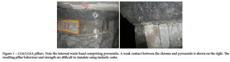
Several publications were recently published on the strength of hard rock pillars in the Bushveld Complex (e.g., Watson et al, 2021; Couto and Malan, 2023; Oates and Malan, 2023). These studies focussed mostly on the UG2 reef and only to a limited extent on other hard rock reef types such as the Merensky Reef or the manganese pillars in the Northern Cape (Watson et al, 2008; Wessels and Malan, 2023). Almost no work has been published on the strength of pillars in excavations exploiting the other chromitite bands such as the MG1, MG2, and the LG6/LG6A package. The strength of these pillars is unknown and the hard rock industry still uses the Hedley and Grant (1972) formula for the design of bord and pillar layouts (Malan and Napier, 2011). The so-called K-value in this power-law strength formula was historically assumed to be a third of the uniaxial compressive strength (UCS) of the pillar material (K= ¹/₃ UCS). The difficulty with the LG6/LG6A pillars is that these pillars are comprised of different rock materials as illustrated in Figure 1. The LG6A chromite is the upper layer and the LG6 is against the footwall. The two chromitite bands are separated by an internal waste band of pyroxenite. These rock types have different UCS values. The contacts between the chromitite may be frozen or consist of weak layers as demonstrated in Figure 1. These weak contacts are known to play a dominant role in the pillar failure mechanisms (Couto and Malan, 2023; Els and Malan, 2023). It is therefore meaningless to use the historic assumption of K= ¹/₃ UCS for these pillars.

A case study of LG6 pillar strength is described by Wesseloo and Swart (2000). They calculated the factor of safety for two sections in an LG6 mine. The one section was subjected to a large collapse in 1960. They analysed 203 pillars in total, of which 90 were failed. This is a valuable database, but the authors of this paper unfortunately did not have access to this specific data. Wesseloo and Swart (2000) concluded from a statistical analysis that the conventional pillar design methodology is not acceptable. As an alternative, they suggested the use of the 'critical factor of safety concept used by Salamon and Munro (1967). From their back analysis, they indicated that the pillar strength is better approximated by a linear formula with a K-value of 39 MPa.

Numerical modelling, using inelastic constitutive models, may be of some value in estimating the pillar strength, but this approach is problematic and risky. It is not clear what constitutive model will best describe the pillar material, as these models are extremely difficult to calibrate and the partings and joints can often not be accurately represented in the continuum codes. Calibration of the discontinuum inelastic codes is also extremely difficult. Malan and Napier (2011) already raised some concerns regarding the use of numerical modelling with appropriate failure criteria to determine pillar strength. For LG6 pillars, Joughin et al (2000) adopted a risk-based approach and two-dimensional modelling using the code PHASE². The advantage of using the finite element approach was that the two chrome layers and the pyroxenite middling could be explicitly modelled. The authors used a Hoek-Brown strength model and the pyroxenite was simulated to be more competent than the chromitite. A historical area of a large collapse and a new mining area were simulated. The modelling indicated that the chromitite controlled the failure of the pillars and the results agreed well with the actual pillar failures observed in the different areas underground. It should be noted, however, that the models used to simulate the failure were two-dimensional and ideally three-dimensional models of the actual pillar layout and geometries should be studied.

A recent example illustrating the risk of inelastic modelling was published by Le Bron et al (2024). The authors proposed the concept of 'pillar load inversion and FLAC3D modelling was done. Elastic modelling will predict high stress at the pillar edges and less in the centre of the pillar. When the edges of the pillar fail, the pillar load is transferred to the confined core. With progressive failure, the stress profile changes from being higher near the pillar edge to a peak in the centre. This defines the 'pillar load inversion'. The strain at failure for laboratory specimens was then used by the authors to determine if a pillar is failed or not. The difficulty is that a Mohr-Coulomb constitutive model without strain softening was used and the reason given in the paper is that: 'For strain-softening to be attempted applying this approach, one would need post-peak residual strength properties. The associated friction angle and cohesion at the residual strength would have to be determined by running sensitivity analyses until representative residual strength parameters are obtained. This information is not available, which is why the Mohr-Coulomb Constitutive model was run. This approach may be questioned. A case study presented in the paper was pillars in the LG6 chromitite seam at depths of 370 m to 500 m below the surface. It is concluded that at a depth of 370 m below the surface, the 8 m x 8 m pillars will remain stable, whereas pillars at 500 m depth are predicted to experience full pillar load inversion and potential failure. These conclusions are based on a Mohr-Coulomb model with no strain softening, which may not be appropriate. The effect of possible weak contacts, as illustrated in Figure 1, was also not simulated. The constitutive model is therefore possibly poorly defined and the modelling results need to be confirmed using underground observations.

This current manuscript explores the alternative approach of the back-analysis of actual LG6/LG6A mining layouts using displacement discontinuity codes to simulate the average pillar stresses on a mine-wide scale. Observations of the actual pillar behaviour are a critical component of this methodology. This allows for the building of a database of actual pillar behaviour and it attempts to mimic the benefit Salamon and Munro (1967) had with a good pillar database. From the modelling, if the simulated pillars are still intact, a 'minimum' K-value can be estimated. In 2009, the second author conducted a study of LG6/LG6A pillar strength at a mine close to Rustenburg. No pillar spalling was observed at a depth of 200 m, even for these very small pillars. From the numerical back-analysis, it was found that the conservative estimate is K > 57.5 MPa. The mine subsequently adopted a K-value of 57.5 MPa and the mining to date indicated a stable pillar environment. Following a similar approach, additional strength data for LG6/LG6A pillars are presented in the paper. This modelling approach was also used by Oates and Malan (2023) for UG2 pillars. The displacement discontinuity method can nevertheless lead to erroneous pillar stress simulations if the user does not have a good understanding of the numerical codes (Napier and Malan, 2011). A secondary objective of the paper is to give some guidelines to inexperienced users who attempt to use this methodology to estimate pillar strength. The effect of element sizes and simulating the effect of the surface for shallow pillars are illustrated using two different boundary element codes. The need for actual pillar observations and an iterative design process, which cycles between modelling and observations, is also emphasized.

 

Aspects to consider when estimating hard rock pillar strength

Owing to the uncertainty in pillar strength and the spatial variability of rock mass strength, several aspects need to be considered. The section below was compiled to assist rock engineering practitioners in this regard.

> The empirical Salamon and Munro (1967) approach for coal strength has been very successful and this simple equation is still used five decades later. Calibrating the power-law strength equation was possible as they collected a good database of intact and failed coal pillar cases. Unfortunately, similar databases are currently not available in the hard rock mining industry for all the different reef types. Efforts should therefore be made to collect as much pillar data as possible.

> The researchers advocating numerical modelling as a much-improved method to determine pillar strength need to consider the historic success of empirical methods. Examples are the empirical data used to determine stable spans and the coal pillar strength formula. Furthermore, inelastic numerical models can be difficult to calibrate owing to the large number of parameters. Selection of an appropriate constitutive model is difficult and an accurate representation of the discontinuities and their strength in the pillar can be problematic. A further problem is the high costs for the licenses and the difficulty of becoming an experienced user of some of the complex codes. For these modellers, a risk is that it may result in a cognitive bias that involves an over-reliance on a familiar modelling tool (Maslow, 1966). This is often quoted as 'If the only tool you have is a hammer, it is tempting to treat everything as if it were a nail'. Although displacement discontinuity boundary element codes are used below, it should be emphasized that other modelling codes should also be considered if the particular pillar problem requires alternative modelling techniques.

> The limitations of the various numerical modelling codes should be considered. Displacement discontinuity codes are well suited to simulate large-scale mining layouts containing a large number of irregular pillars. The effect of the surface for shallow excavations can be easily simulated. The drawback of these codes is that it cannot simulate the detailed pillar failure mechanisms. In contrast, finite difference and finite element codes can simulate the pillar failure mechanism in detail (provided an appropriate constitutive model is selected). The drawback of these codes is that it cannot simulate a large assembly of irregular pillars. Calibration of the complex constitutive models is also exceedingly difficult as it often includes a large number of parameters. The models are typically restricted to a single pillar only. Furthermore, for all types of codes, numerical modelling aspects, such as element size, may affect the simulated results and the modeller must be familiar with the limitations of the solution method and the particular code. The effect of element size for average pillar stress (APS) calculations in displacement discontinuity codes is demonstrated in the following.

> Malan and Napier (2011) concluded that neither empirical techniques nor numerical modelling can be used in isolation to provide a solid basis to predict pillar strength. Both these techniques should therefore be used when addressing pillar design problems to obtain the best possible insights. This was recently also advocated by Le Bron et al (2024) and they proposed a hybrid methodology, which includes both the empirical method and numerical modelling (although the empirical method is not discussed in their paper).

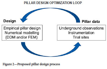
> Owing to the uncertainty in pillar strength and the possible variability of rock mass strength in different areas of the mine, an iterative design process needs to be adopted. This is illustrated in Figure 2. As an illustration, if pillar sizes are reduced after conducting a numerical back-analysis study of the existing pillars and estimating a different K-value, a trial section needs to be established. Observations and possibly monitoring should be conducted in this section. Further numerical modelling is then required to determine if additional optimisation of the pillars is possible.

> For empirical pillar design, there is uncertainty about whether to adopt a power-law strength formula or a linear strength formula (Ryder and Jager, 2002). Salamon and Munro (1967) noted: The volume and shape of square pillars are completely defined by their width (w) and height (h). The most commonly-occurring pillar strength formula in the literature is a simple power function composed of these variables.' The last sentence in the quote is of particular importance. The equation selected by Salamon and Munro (1967) was therefore 'the most commonly-occurring pillar strength formula in literature. For the hard rock strength formula, Hedley and Grant (1972) used the same references of the 1940s and 1950s, as well as Salamon's work, to motivate the use of a power-law equation. The exponents of the Hedley and Grant formula appear to be a reasonable approximation to account for variations in pillar width and height and it is recommended that this be retained for now, unless good laboratory and underground data can be obtained to indicate otherwise. This equation is also adopted in this paper.

> When conducting a back-analysis of pillar strength, it may be difficult to find failed pillars in the existing bord-and-pillar layouts. As a useful alternative, it is recommended to search for the smallest pillars in the deeper sections of these layouts. The average pillar values will be the largest on these pillars. If the Hedley and Grant equation is adopted, the unknown value is the rock mass strength K in the equation below.

 

 

 

Equation [1] can be rearranged to give:

A good estimation of the 'minimum' K-value can be obtained by using the simulated APS value in the previous section as the 'minimum' pillar strength. If it is assumed that σ_s=APS and K = K_min, Equation [2] can be written as:

This equation is used in the following in the back-analysis of the pillar stresses.

 

Numerical modelling aspects when estimating average pillar stress

The displacement discontinuity boundary element method to simulate tabular layouts has been popular in South Africa since the early 1970s (Plewman et al., 1969; Deist et al., 1972; Ryder and Napier, 1985; Napier and Stephansen, 1987). Unfortunately, the expertise to develop these codes in South Africa has now almost disappeared. A good understanding of the limitations of the method is currently limited to a handful of individuals and only limited numerical modelling is conducted on the mines. Two different boundary element codes were used for this study, namely MAP3D and TEXAN. This paper is a useful verification of the two codes and it was expected that similar pillar stresses would be simulated by these codes. TEXAN is a displacement discontinuity code and it has been described in many earlier papers (Malan and Napier, 2006; Napier and Malan, 2007). In MAP3D, the user can use both displacement discontinuity elements for tabular excavations and fictitious force elements to simulate large excavations (Wiles, 2024). The simulations for this study were nevertheless limited to displacement discontinuity elements to simulate bord-and-pillar layouts. Of particular interest was the effect of element size on average pillar stress (APS) and simulating the effect of the surface when analysing shallow excavations.

When adopting the displacement discontinuity method, the surface of the problem space needs to be divided into several sub-regions or elements. A simplified functional form of the displacement discontinuity distribution within each element needs to be adopted. In the early applications of the method, such as in MINSIM-D, this function was assumed to be a constant within each element and a square element shape was adopted. Ryder and Napier (1985) noted that the magnitudes of the solved displacement discontinuity values are affected by the element size when using this approach. The proposed solution was to use 'partially mined elements' and the excavation outlines were shifted by the 'quarter grid correction. This allowed for accurate far-field stress distributions to be computed, that are independent of element size. A major shortcoming of this approach was that it became difficult to estimate average pillar stresses as the pillar outlines were now approximated. The approach was nevertheless adopted as the early displacement discontinuity codes were developed for the gold mines, and the important parameters to compute were stope convergence and energy release rate (ERR). The need to simulate the average pillar stress of a large number of small pillars in bord and pillar layouts only became a requirement in later years. This resulted in the development of the TEXAN code that included higher-order triangular and quadrilateral elements (Napier and Malan, 2007). MAP3D also allows for the use of higher-order elements. The code allows for the selection of 'linear' or 'quad' in the analysis options, otherwise, the displacement discontinuities are treated as constant values. As stated in Wiles (2024), for the linear option, the stress or displacement discontinuity is distributed over the boundary elements using a linear order polynomial distribution. For the 'quad' option the stress or displacement discontinuity is distributed over the boundary elements using a quadratic order polynomial distribution. All simulations in this paper were performed by using constant displacement discontinuity elements.

For the TEXAN code, Napier and Malan (2011) conducted a study on the effect of element size on APS. Errors can arise depending on the choice of element size and the element shape in a geometrically complicated layout. Typically, coarse constant strength displacement discontinuity elements underestimate the correct APS value. Interestingly, for a two-dimensional pillar problem, the simulated APS is very close to the analytical solution if the element size approaches zero. This was also illustrated for a circular pillar. The authors proposed extrapolation techniques and simulations with different element sizes to obtain better approximations of the correct APS values. They nevertheless recommended that this approach must be treated with caution for tabular excavations and noted: 'Unfortunately, there are no simple numerical solutions to this problem.' In practice, a pragmatic solution is simply to use the smallest possible element sizes that will not be too computationally arduous. Unfortunately, when reviewing previous papers where the APS values of pillars were computed, it is typically not known what element sizes the authors used in the simulations. For example, Wesseloo and Swart (2000) describe a case study of a large pillar collapse in a LG6 mine in 1960. The APS values of these pillars were calculated using BESOL/MS (a displacement discontinuity code), but the authors do not specify the element sizes used.

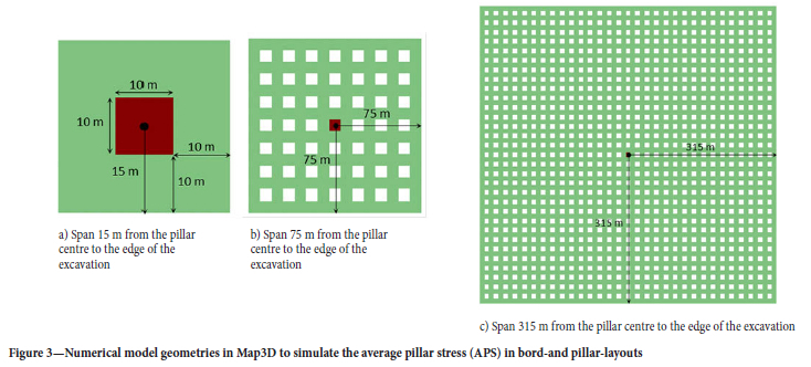
The effect of element size on APS has never been demonstrated for the MAP3D code and this could have led to an underestimation of pillar stress in many previous pillar simulations in South Africa. For this study, a number of simulations were therefore conducted to investigate this effect. It was found that the selected 'element length' and the overall size of the excavation ('mining span') will affect the simulated APS. To investigate the effect of element size on the simulation of bord-and-pillar layouts and how the simulated APS relates to tributary area theory (TAT), several simulations were conducted. Different bord-and-pillar layouts were constructed in Map3D using square 10 m x 10 m pillars. The bord widths and holings between the pillars were 10 m and the simulated depth was 1000 m. The density of the overburden was assumed to be 3100 kg/m³. During the setup of the numerical models, fixed element widths (aL) of 1, 2, 5, and 10 were used for the pillar and the bords. The resulting number of elements and the element lengths are given in Table I. Note that these were the actual element lengths and, for the smaller elements, it was different to the specified AL parameter. It is not clear how the meshing algorithm uses the various parameters. Several geometries of increasing total span were simulated. This is illustrated in Figure 3. The number of pillars in each geometry increased as the overall span increased. The pillar APS value of interest was that for the pillar in the centre of the layout.

 

 

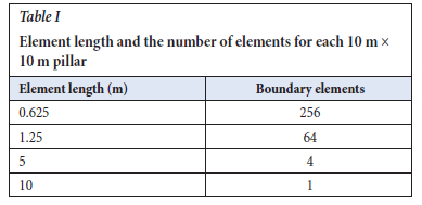
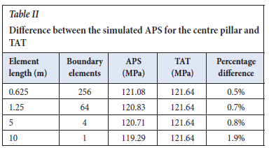
Care should be exercised when computing the average pillar stress in Map3D. The author found that to obtain the correct value, the normal stress on the displacement discontinuity for each element should be exported to Excel and the average should then be computed. The calculated values for the centre pillar for various spans and element sizes are shown in Figure 4. It is clear from these results that large spans and many pillars are required for the APS value to approximate the tributary area value (TaT). If it is required that the difference in average pillar stress at the centre pillar be less than 1% of the TAT value as illistrated in Table II, the element length should be equal to or less than 1/2 of the smallest width of the pillar and the minimum half-span required was found to be 300 m. As a crude rule of thumb, the minimum mining half-span should be 30 times the pillar width for regular bord-and-pillar layouts for Map3D simulations.

 

 

 

 

It should be noted that MAP3D uses quadrilateral elements to accurately mesh irregular pillars. The meshing of a square pillar and an irregular pillar is shown in Figure 5. In TEXAN, triangular elements are used to accurately mesh irregular pillars.

 

 

A further important aspect to consider is shallow conditions. Many of the hard rock bord and pillar layouts are located close to the surface and the average pillar stress will be underestimated if the effect of close proximity to the surface is not accounted for. As described in Napier and Malan (2007), shallow conditions can be simulated by an artificial 'excavation' at the surface position and included in the simulation with the 'real' underground mining excavation. The drawback is long run times and selecting the appropriate extent of the surface excavation is difficult. If large element sizes are used on the surface, this may lead to iterative solution difficulties if the underground excavations are in close proximity. As a more efficient approach, it is possible to use appropriate influence functions that allow for the effect of the surface to be included automatically without requiring the inclusion of the explicit surface. These influence functions were developed for TEXAN and are given in Napier and Malan (2007). In MAP3D a displacement discontinuity plane is typically placed on the surface to simulate the effect of the free surface and this was also done for the Map3D simulations below. The effect of simulating the average pillar stress with and without the free surface is illustrated below for both codes.

 

Back analysis case study to determine the K-value

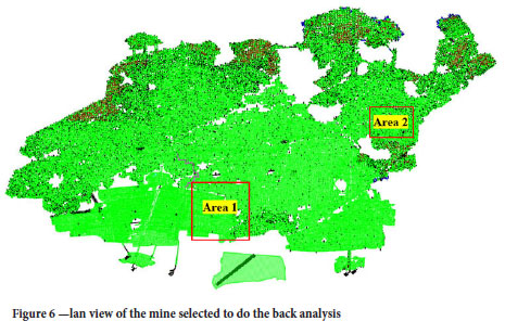
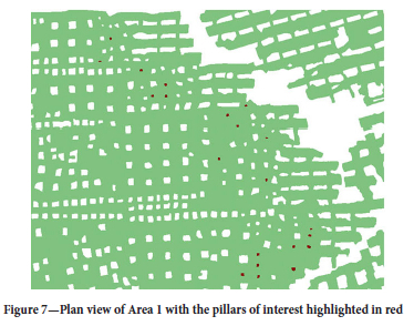
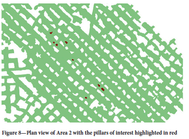
The mine used as a case study is situated in the western Bushveld Complex and is mining the LG6/LG6A chromitite seams. As shown in Figure 1, the LG6 is on average 1.0 m in thickness and overlain by the LG6A, averaging 30 cm in thickness. The internal waste comprising the pyroxenite has an average thickness of 50 cm. As shown in Figure 6, the selected areas for back analysis were Area 1 (last mined in 1991) and Area 2 (mined in 2009). The small pillars in both areas are shown in Figures 7 and 8 and are highlighted in red. A total of 29 pillars were identified that had a width-to-height ratio ranging from smaller than 1 to larger than 3. The mining spans around these pillars were also typically larger than expected. Especially the small pillars in Area 1 are surrounded by large mining spans. It is expected that the stresses acting on these pillars would be larger than for the other pillars at these depths. Area 1 is situated at a mining depth ranging from 75 m to 121 m and in Area 2 the mining depths vary from 190 m to 201 m.

 

 

 

 

 

 

Numerical modelling results

Numerical modelling of Area 1 was done by using both the TEXAN and Map3D codes. A direct comparison of these two codes when simulating average pillar stresses in bord-and-pillar layouts has never before been published. These results are therefore also valuable as a verification of the codes. Area 2 was only simulated with the Map3D code to obtain additional pillar stress data. Note that, for the areas simulated, the pillars of interest are typically small and these are surrounded by larger pillars. The question can be posed if there is any load 'bridging' to the larger pillars and if the numerical modelling results possibly overestimate the load on the smaller pillars. Napier (2023) conducted preliminary numerical modelling results, in which he used special traction discontinuity influence functions that were combined with the displacement discontinuity elements to represent thin beam flexure effects for stiff material layers above the pillars. From this study it was evident that the APS values are lower when there is a stiff overlying layer compared to the case where there is no layer. The modulus of the rock was 70 GPa and 90 GPa for the stiff beam. This modelling illustrated the so-called 'stress bridging' effect in which the stiff layer reduces the average pillar stress values. The example highlights that the presence of significant material property contrasts requires careful assessment when computing average pillar stress values and pillar stability. Ideally, stress measurements are needed in the small pillars to confirm that no stress bridging occurs. For the cases illustrated in Figures 7 and 8, such a modulus contrast was not present in the hanging wall and the rock was a uniform pyroxenite. It was therefore assumed that the simulated stress in this case is a good approximation of the average pillar stress.

 

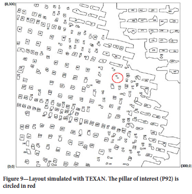
Figure 9 illustrates the area simulated by TEXAN and the pillar shapes are approximated by straight-line polygons. The pillar of interest is highlighted by the red circle. Note that it is a small pillar surrounded by very large spans and it is therefore expected to carry a large stress. The depth is 101 m and the overburden density is assumed to be 3100 kg/m³.

 

 

The simulated results for the pillar of interest (P92) are shown in Figure 10. The pillar size was 5.38 m². Triangular elements were used, so the element size is the average size of the elements in the pillar of interest. Various element sizes and both the finite depth (simulating the free surface) and infinite depth (no free surface) solutions in TEXAN were used. As expected, the APS increases as the element size decreases. This is discussed in detail in Section 3.

 

 

The APS is the y-intercept (zero element size) and for the infinite depth solution it is APS = 76.5 MPa and for the finite depth solution, it is 81.8 MPa. Note that the APS value is approximately 7% higher when simulating the surface and it highlights the importance of considering this for shallow excavations. Also note the effect of element size and the importance to use extrapolation, or at least the smallest practical element sizes, to get a good approximation of the APS value.

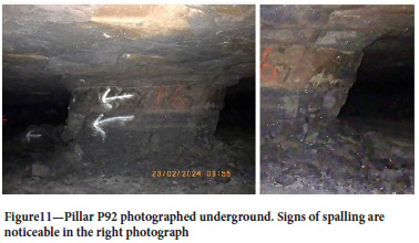
The pillar still appears to be in good condition, but some spalling of the chromitite can be seen (Figure 11). Based on its condition, it is assumed that the factor of safety on this pillar is still higher than unity.

 

 

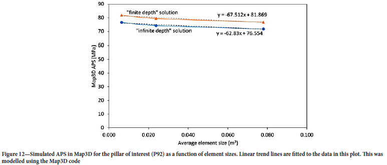
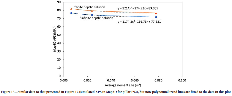
Map3D models of this area were also built and the stress on the same pillar was simulated using different element sizes. The element sizes were smaller than that used for the TEXAN simulations. Different simulations were conducted with a sheet of elements simulating the surface explicitly, and also without simulating the surface. The simulated pillar area was also 5.38 m². The results are given in Figures 12 and 13. These results are encouraging as essentially similar results were obtained for the two codes. For a linear trend line (Figure 12), the infinite depth solution at the y-intercept is APS = 76.6 MPa and for the finite depth solution, it is 81.9 MPa. For a polynomial trend line (Figure 13), the infinite depth solution at the y-intercept is APS = 77.7 MPa and for the finite depth solution, it is 83 MPa. It seems as if Map3D is simulating marginally higher APS values, but this may be caused by the very small elements used.

Map3D was used to simulate the stress acting on the other 28 pillars of interest (both Areas 1 and 2). The surface was explicitly simulated for these runs. These pillars are situated at depths ranging from 75 m to 201 m and the overburden density is assumed to be 3100 kg/m³. The Map3D mesh parameter 'element length' (AL) for these pillars was fixed and was set to 0.5, 0.25 and 0.125 for the different models (these values gave the different element sizes in Figure 12). Figures 14 and 15 indicate the pillar conditions underground for some of the pillars used in the back analysis. In some areas, it was difficult to photograph these pillars due to dust and scalping (sorted waste rock) stored in the back areas.

 

 

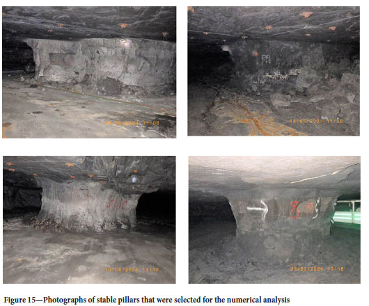
It should be noted that the pillars shown in Figures 14 and 15 are in remarkably good condition for an area that was mined in 1991, taking into consideration possible time-dependent deterioration, jointing, and poor mining. As mentioned, a total of 29 pillars were selected and 28 of these pillars had a width-to-height ratio ranging from larger than 1 to larger than 3. One pillar had a width-to-height ratio of smaller than 1 (Figure 16). In Area 1, the mining spans are larger than expected, with mining spans in some areas greater than 20 m.

 

 

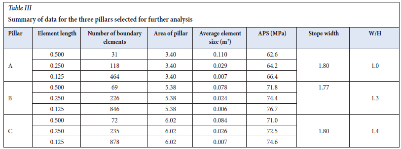
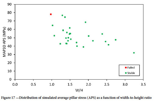
The numerical results are summarized in Figure 17. Based on the underground observations of the pillars and the numerical modelling, three pillars were selected to estimate a K_min value. These pillars are shown in Table III. Note the small w:h ratio, small pillar areas, and large APS values. It can therefore be speculated that these pillars are loaded close to failure.

 

 

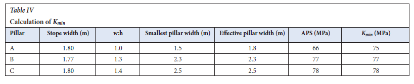
Using the data in Table III and Equation [3], the K_min value for the three identified pillars was calculated. The results are given in Table IV and K = 77 MPa may be a good approximation to determine the pillar strength. Interestingly, this is almost similar to that obtained by Oats and Malan (2023) for the UG2 pillars (K = 75 MPa). This value nevertheless needs to be tested in controlled trial mining sections before it is adopted on a larger scale.

The data collected as well as the pillar strength envelopes for a Hedley and Grant equation with a K-value of 35 MPa and 77 MPa are plotted in Figure 18. The historic assumption of K = 35 MPa was far too conservative. Only one failed pillar is in the database, however, and additional data needs to be collected.

 

Conclusions

This case study indicates that the current used K-value for the LG6/ LG6A pillars of 35 MPa may be too conservative in some areas. This is adversely affecting the extraction ratio in the western Bushveld Complex. From the back analysis done on small pillars, a K-value of 77 MPa for LG6/LG6A seems to be more appropriate for the area studied. This needs to be tested in a trial mining section before it can be implemented on a larger scale. Careful observations and further modelling of this trial section must be done to validate the new K-value. This is particularly important considering that previous workers estimated a K-value of 39 MPa for a linear formula for LG6 pillars at an unknown mine. The value of displacement discontinuity modelling to obtain better estimates of pillar strength is nevertheless clear from the study. Users should be careful with the selection of element sizes, however, and the surface must be explicitly simulated if the excavations are close to the surface.

 

Acknowledgements

The authors would like to thank Samancor Chrome Ltd. for permission to publish this data and for the opportunity to use Samancor equipment and numerical modelling software.

 

References

Couto, P.M., Malan, D.F. 2023. A limit equilibrium model to simulate thwe large-scale pillar collapse at the Everest Platinum Mine. Rock Mechanics and Rock Engineering, vol. 56, pp. 183-197.         [ Links ]

Deist, F.H., Georgiadis, E., Moris, J.P.E. 1972. Computer applications in rock mechanics. Application of Computer Methods in the Mineral Industry. Proceedings of the 10th International Symposium, Johannesburg. pp.259-266. https://www.saimm.co.za/Conferences/Apcom72/000b-Contents.pdf        [ Links ]

Els, R.P., Malan, D.F. 2023. Calibration of the limit equilibrium pillar failure model using physical models. Journal of the Southern African Institute of Mining and Metallurgy, vol. 124, no. 5, pp. 253-263.         [ Links ]

Hedley, D.G.F., Grant, F. 1972. Stope-and-pillar design for the Elliot Lake Uranium Mines. Bulletin of the Canadian Institute of Mining and Metallurgy, vol. 65, pp. 37-44.         [ Links ]

Joughin, W.C., Swart, A.H., Wesseloo, J. 2000. Risk based chromitite pillar design. SANIRE 2000 Symposium, "Keeping it up in the Bushveld". https://www.researchgate.net/publication/262767130_Risk_based_chromitite_pillar_design_-_Part_11_Non-linear_modelling        [ Links ]

Le Bron, K.B., Gardner, L.J., Van Zyl, J. 2024. Beyond the empirical pillar design method: The strain criterion and the pillar load inversion concepts. Journal of the Southern African Institute of Mining and Metallurgy, vol. 124, no. 5, pp. 293-302.         [ Links ]

Malan D.F., Napier, J.A.L. 2006. Practical Application of the Texan Code to Solve Pillar Design Problems in Tabular Excavations, SANIRE Symposium "Facing the challenges", Rustenburg, pp. 55-74.         [ Links ]

Malan, D.F., Napier, J.A.L. 2011. The design of stable pillars in the Bushveld mines: A problem solved? Journal of the Southern African Institute of Mining and Metallurgy, vol. 111, pp. 821-836.         [ Links ]

Maslow, A.H. 1966. The Psychology of Science: A Reconnaissance. Harper & Row. pp. 15. https://fumaca.pt/wp-content/uploads/2022/12/The-Psychology-of-Science-A-Reconnaissance-PDFDrive-.pdf        [ Links ]

Napier, J.A.L. 2023. Unpublished numerical modelling.         [ Links ]

Napier, J.A.L., Malan, D.F. 2011. Numerical computation of average pillar stress and implications for pillar design. Journal of the Southern African Institute of Mining and Metallurgy, pp. 837-846.         [ Links ]

Napier, J.A.L., Malan, D.F. 2007. The computational analysis of shallow depth tabular mining problems, Journal of the Southern African Institute of Mining and Metallurgy, vol. 107, pp. 725-742.         [ Links ]

Napier, J.A.L., Stephansen, S.J. 1987. Analysis of Deep-level Mine Design Problems Using the M1NS1M-D Boundary Element Program, APCOM 87. Proceedings of the Twentieth International Symposium on the Applications of Computers and Mathematics in the Mineral Industries, vol. 1: Mining. Johannesburg, SAIMM. pp. 3-19.         [ Links ]

Oates, T.E., Malan, D.F. 2023. A study of UG2 pillar strength using a new pillar database. Journal of the South African Institute of Mining and Metallurgy, vol. 123, no. 5, pp. 265-273.         [ Links ]

Plewman, R.P., Deist, F.H., Ortlepp, W.D. 1969. The development and application of a digital computer method for the solution of strata control problems. Journal of the Southern African Institute of Mining and Metallurgy, vol. 70, pp. 33-44.         [ Links ]

Ryder, J.A., Jager, A.J. 2002. A Textbook on Rock Mechanics for Tabular Hard Rock Mines. Safety in Mines Research Advisory Committee, Johannesburg, pp. 397-440.         [ Links ]

Ryder, J.A., Napier, J.A.L. 1985. Error analysis and design of a large-scale tabular mining stress analyser. The 5th International Conference on Numerical Methods in Geomechanics, Nagoya, Japan. pp. 1549-1555.         [ Links ]

Salamon, M., Munro, A. 1967. A study of the strength of coal pillars. Journal of the South African Institute of Mining and Metallurgy, vol. 67, pp. 56-67.         [ Links ]

Watson, B., Ryder, J.A., Kataka, M.O., Kuijpers, J.S., Leteane, F.P. 2008. Merensky pillar strength formulae based on back-analysis of pillar failures at Impala Platinum. Journal of the Southern African Institute of Mining and Metallurgy, vol. 108, pp. 449-456.         [ Links ]

Watson, B.P., Theron, W., Fernandes, N., Kekana, W.O., Mahlangu, M.P., Betz, G., Carpede, A. 2021. UG2 pillar strength: Verification of the PlatMine formula. Journal of the Southern African Institute of Mining and Metallurgy, vol. 121, pp. 449-456.         [ Links ]

Wessels, D.G., Malan, D.F. 2023. A limit equilibrium model to simulate time-dependent pillar scaling, Rock Mechanics and Rock Engineering, vol. 56, pp. 3773-3786.         [ Links ]

Wesseloo, J., Swart, A.H. 2000. Risk based chromitite pillar design - application of the locally empirically derived pillar formula, SANIRE 2000 Symposium, "Keeping it up in the Bushveld".         [ Links ]

Wiles, T.D. 2024. Map3D User's Manual - Version 68.         [ Links ]

 

 

Correspondence:
P.J. Le Roux
Email: Jaco.LeRoux@samancorcr.com

Received: 22 Aug. 2022
Revised: 20 Oct. 2024
Accepted: 22 Oct. 2024
Published: November 2024