Velocity measurement in a hydrodynamic torque converter

 

 

P.J. Strachan^I; T.W. von Backström^II

^IDepartment of Mechanical Engineering, University of Stellenbosch, Private Bag XI, Matieland, 7602 South Africa
^IIDepartment of Mechanical Engineering, University of Stellenbosch, Private Bag XI, Matieland, 7602 South Africa

 

 

---

ABSTRACT

An experimental torque converter in which flow characteristics could be both observed and measured was manufactured and tested. Flow visualisation was carried out by means of fluorescent tufts, air bubbles and polystyrene particles, and from these visualisations, flow velocities and angles were determined by using video and still photography. Differential pressure probes were used for direct measurement of flow velocity at different stations in the flow path. Agreement between results obtained by these different methods was good. The torque converter performance was also simulated by means of a o ne-dimensional hydro-dynamic model, and acceptable overall agreement was obtained between measured parameters and the model's results.

---

 

 

Introduction

In previous work¹ the description was given of a one-dimensional computer program for analysing torque converter performance, in which much of the empiricism in the input data, found in similar models, had been removed and replaced by empirical equations and loss models built into the program. Due to the model's need for very detailed input data, particularly relating to geometry, its efficacy could only be validated against two sets of published results, namely those by Lamprecht² and Jandasek.³ In both cases the improvement in accuracy over existing models was significant. In order to further validate the model and to evaluate torque converter characteristics, an experimental torque converter was developed in which the flow could be observed and measured.⁴ In addition, the dimensions of the experimental torque converter could be accurately measured and used as input to the model.

This paper describes the apparatus and compares the measured results with those determined by the one-dimensional hydrodynamic model.

 

Description of the apparatus

Torque converter test rig

The test rig (Figure 1) was a universal facility capable of testing a variety of hydrodynamic drives such as torque converters and fluid couplings. It consisted of two sets of identical 5.5 kW, variable speed (0-3 000 rpm) electric motors and 4.45:1 step-down gearboxes, which could be connected to the input and output shafts of either a torque converter or fluid coupling. For reasons given later, the experimental torque converter utilised in the experiment was only operated in stall, and consequently only the input drive system of the test rig was used. The test rig provided controlled, independent and infinitely variable input speed, which was measured by a proximity transducer, excited by a 60-tooth disc attached to the input shaft. Torque measurement was by means of a specifically developed contact less torque transducer.

 

 

Experimental torque converter

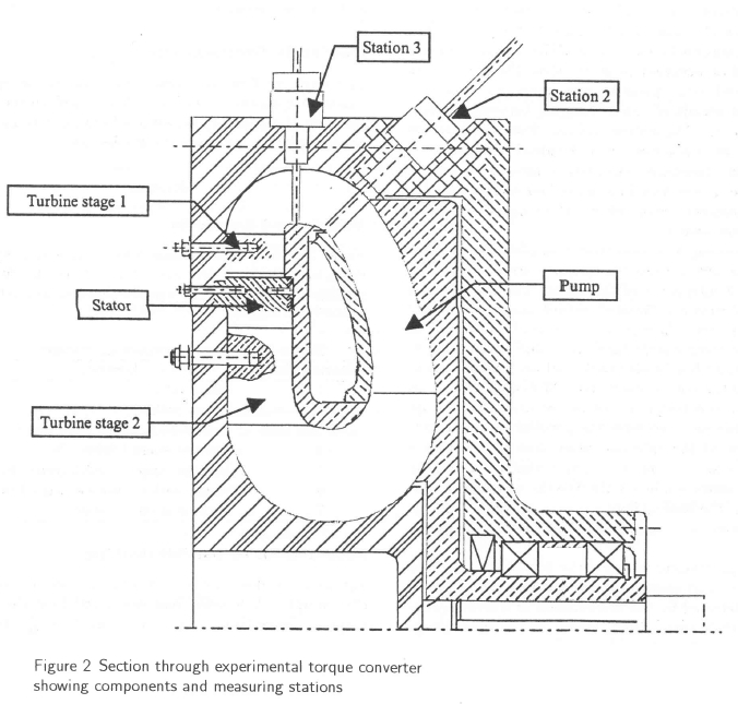
The experimental torque converter (Figure 2) was a full-size model of a commercial unit for which manufacturing drawings were available. The torque converter had a single stage pump with a two stage turbine and in its commercial form was capable of transmitting 1 500 Nm of torque at 2 600 rpm, an equivalent power of approximately 410 kW. In order to reduce the power requirement for laboratory purposes, water was used as the working fluid and therefore to maintain dynamic similarity a lower rotational speed was required. Assuming kinematic viscosities of 6.0 X 10^-6 m²/s for a typical hydraulic transmission fluid at a temperature of 100° C, and 0.66 x 10^-6 m²/s for water at a temperature of 40°C, the speed ratio for constant Reynolds number should be 10:1. Therefore an input speed of 260 rpm was used on the test rig, resulting in a maximum torque of 68 Nm and a maximum power of about 2 kW.

In order to permit visual observation of the flow conditions, part of the torque converter casing was manufactured from clear perspex. This exposed the two stages of the turbine, the stator and the inlet to the pump. As it would also be necessary to measure flow velocity at various stages in the flow path, it was decided to maintain the output shaft stationary and thus to operate the torque converter in stall. Although this would obviously limit the range of results obtained, it would greatly simplify measurement. In addition, the stall point of a torque converter is probably its most important operating situation and thus it was considered that results obtained at this condition would have the most significance.

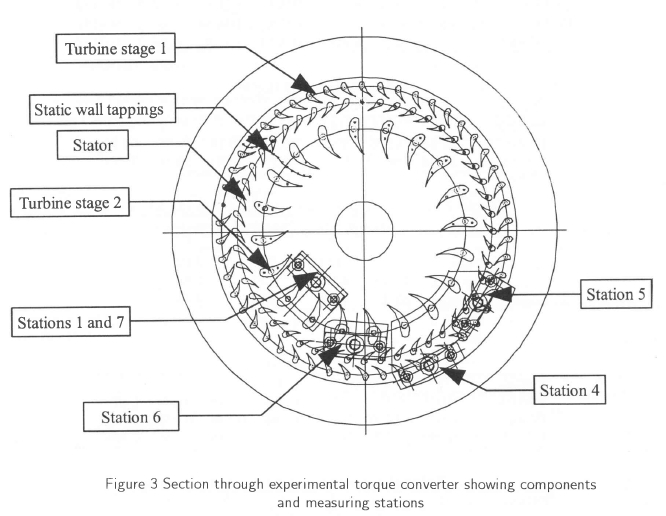
As shown in Figures 2 and 3, foot plates for the probe traversing mechanisms were provided at 6 different positions on the torque converter housing, permitting flow measurement by directional pressure probes at 7 different locations in the flow path. These were at the entrance to (location 1) and exit from the pump (2), midway in the channel between the pump exit and the entrance to turbine stage 1 (3) and at the entrances (4,6) and exits (5,7) of the two turbine stages. As can be seen from Figures 2 and 3, locations 1 and 7 were at the same position on the torque converter housing. In addition, static wall pressure tapings were provided at 15 locations between the entrance to turbine stage 1 and the exit from turbine stage 2 as also shown in Figure 3.

Instrumentation

Two types of directional pressure probes were used to measure the total and static pressure and determine the flow velocity and direction. Two of the probes were of the 3-hole type and one was of the 5-hole type. The probes were mounted on a traversing mechanism permitting translation and rotation. All the probes were calibrated in a water tunnel in which the flow velocity was measured by means of a flow contraction. The probes and their traversing mechanism were fitted to the side wall of the tunnel and the water velocity was varied between 1 m/s and 9 m/s. The dynamic pressure of the flow was determined from the difference between the total and quasi-static pressuras recorded by the probes.

Two electronic differential pressure transducers were used to measure the pressures recorded by the probes. The pressure transducers had a nominal differential pressure of 0.01 bar, and an accuracy of better than 1%. The probes were connected to the pressure transducers by a series of valves, which permitted rapid changing between different probe positions. The output voltage from the pressure transducers was measured on a standard voltmeter. A third pressure transducer was used to measure the static wall pressure at the locations described above. All the pressure transducers were calibrated by means of a standard water manometer.

A thermocouple thermometer was placed in the flow circuit at the outlet from the torque converter pump to measure the temperature of the water. The thermometer was supplied with a calibrated output, and temperature readings were given directly from a digital voltmeter. In order to limit temperature build-up in the water, a circulating system with a header tank and an external pump was fitted to the torque converter. Water was taken off and added to the torque converter at diametrically opposed locations so as to have the greatest cooling effect. A further use of the external pump was to maintain a ■slight over-pressure on the torque converter to prevent the ingress of air through minor leaks into the unit during testing. However, the cooling flow was shut off when readings were taken to ensure a mass flow balance within the torque converter.

The torque transducer was of the non-contactless type and was developed specifically for the test rig. Applied torque was detected by the deformation of a strain gauge mounted on the rotating shaft. Power for the strain gauge was provided by a remote external power pack and was transmitted inductively between two coils, one mounted on the non-rotating transducer housing and the other mounted on the rotating shaft. The signal from the strain gauge was amplified within the transducer and transmitted to a digital display via capacitative decoupling through concentric rings on the rotating shaft and in the stationary transducer housing.

Flow visualisation techniques

Three techniques were used for visualisation of the flow.

Fluorescent cord of 0.1 mm in diameter was cut into short tufts and attached to the outlet of the pump and to the inlet to turbine stage 1. By means of stroboscopic light the position of the tufts could be determined, giving an indication of the direction and status of the flow. Air bubbles were introduced into the flow stream through the 3-hole probe located in the channel between the pump and turbine stage 1. At certain speeds the path of the bubbles gave a clear indication of the flow direction.

At higher speeds, polystyrene chips of approximately 2 mm diameter, 2 mm in length and having a density 2.8% greater than that of water, were admitted into the unit through the water inlet. A good indication of flow direction was obtained and recorded by means of both video and still photography.

Flow angle determination

The angle of flow was measured from photographs by means of a digital protractor. This worked on the principle of an electronically sensed pendulum and had a digital readout with an accuracy of 0.05 degrees.

 

Results

Velocity and flow angle

Table 1 defines the stations where measurements were taken and Tables 2 toll show the test results with comparable values from the one-dimensional hydrodynamic model (1-D Model).

 

 

 

 

Measurement by particle tracking

Approximate flow angles were directly determined from photographs. Velocities were calculated from the photograph exposure time, which was varied from s to s, and the length of the particle tracks. Since it was difficult to judge how far the particles were from the walls of the flow passages, where large deviations from the mean were expected, these values, summarized in Tables 2 and 3, could only serve as checks of the flow some distance from the wall. Other factors influencing the accuracy of flow velocity measurement by particle tracking are the finite size of the particles and the deviation of their densities from that of water.

 

 

Measurement by dynamic pressure probes

Flow angles were determined by turning the probes until the quasi-dynamic pressures on the left and right sides of the probe were equal. The quasi-dynamic pressure was the difference between the probe stagnation pressure and the side hole pressure. Since the model had been designed with all the probe axes in the horizontal plane, flow angles were easily determined by means of the digital protractor. The convention for the flow direction was according to Figure 4 with the observer always on the outside of the flow circuit and looking in. Wakes of upstream blade rows would have had a large influence on the accuracy of the flow measurement by means of probes. The effect of blockage and the shear effects would have had an effect on the velocity magnitude and direction.

 

 

Discussion of results

Velocity profiles

The absolute velocity profiles, as shown for the different stations in Figures 5 to 10, were fairly uniform, with a tendency for the higher velocities to occur on the inside of the flow circuit. There were, however, visual indications of flow separation on the inner wall of the section between the exit from turbine stage 2 and the inlet to the pump, although this was not apparent from the probe readings.

 

 

 

 

 

 

 

 

 

 

 

 

Mean absolute velocities

The mean velocities were calculated as the numerical averages of the values measured by the probes at each station. It is clear from Table 2 that the agreement between the particle tracking results (Particle) and the dynamic pressure probe (Probe) results was good, except at station 4, the turbine stage 1. Despite careful checking no adequate explanation could be found, but the most likely cause was the effect of pitch angle on the probe, coupled with unsteadiness caused by the passing of the pump impeller blade wakes. Agreement between the probe and the one-dimensional model (1-D Model) results was not as good, although the differences were acceptable, apart from stations 1 and 7, the pump inlet and turbine stage 2 outlet, due probably to the difference in radial location for these stations between the Probe and the 1-D Model.

Mean flow angles

The mean flow angles, as given in Table 3, were determined in the same way as the mean velocities. Differences between angles determined by the two methods varied from 4% to 19%, the latter at station 4. Similar to the velocity results, the probe output may have been influenced by upstream wakes. Agreement between the Probe and the 1-D model results was again acceptable, with the exception again of station 4, where the difference was 51%.

Meridional velocities

The agreement between the two methods of measuring the meridional velocity, as shown in Table 4, was good, with the exception again at station 4 where the difference was 32%. Good agreement was also found between the model and the probe results, except at stations 4 and 7, where the differences were 40% and 26%.

 

 

Mass flow

The mass flow circulation through the experimental torque converter (Table 6), as calculated from the product of the meridional velocity (Table 4), flow area (Table 5), and density (assumed to be 996 kg/m³), should have been virtually constant at all measuring stations, as it effectively was for the 1-D hydrodynamic model. The typical standard deviation in mass flow (shown in Table 7) was however only about 2% for the experimental methods, or nearly 9% for the probe, if the doubtful measurements at stations 4 and 7 are included.

 

 

 

 

 

 

Tangential velocities

For practical reasons, the particle and probe results could not always be determined at the same radius as the 1-D model, as can be seen in Table 8. However agreement between the particle and probe methods was reasonable, with differences of between 5% and 14%, but both these results differed markedly from those for the one-dimensional model.

 

 

Angular momentum per unit mass flow

The angular momentum per unit massflow was determined from the product of the tangential velocity (Table 9) and the radius (Table 8) at the measuring point. Once again the agreement between the measuring methods was fair, but results from both methods differed from the one-dimensional model.

 

 

Torque

The torque exerted on or by each member is the product of the mass flow through the member and the change in angular momentum per unit massflow across the member. From Table 11 it can be seen that differences between the Probe and the 1-D Model varied between 1% for the turbine stage 1 and 13% for the stator.

 

 

 

 

The pump impeller torque at 260 rpm as measured by the torque transducer was 24.5 Nm, about 2.5% higher than predicted by the one-dimensional model and about 7% lower than that calculated from the measured angular momentum fluxes. Torque at other speeds is shown in Figure 11.

 

 

Von Backstrom and Venter⁵ also determined the torque exerted by the second turbine by means of blade surface static pressure measurements. If their results are corrected for the fact that their pressure taps did not cover the rearward 20% of the blades, their measured torque for turbine stage 2 comes to 33.7 Nm at 260 rpm, about 6% higher than that deduced from the probe readings. It appears that the torque prediction by the 1-D model is low by 5 to 8%. According to the laws of similarity for turbo-machinery, the torque should vary with the square of the speed, but the coefficients of the second degree equation are influenced by Coulomb friction, which is independent of speed, laminar friction, which is directly proportional to speed, and Reynolds number effects, which cause a deviation from the quadratic relationship between torque and speed.

 

 

Conclusion

An experimental torque converter was manufactured and tested, in which flow characteristics could be observed and measured, in order to assist in the validation of a comprehensive one-dimensional hydrodynamic model. In general, good agreement was found between experimental results obtained both by particle tracking and dynamic pressure probes. In some cases, particularly at station 4, the entrance to turbine stage 1, the differences were unaccept-ably large, but the high level of swirl resulting from the complex geometry increased the difficulty of measurement here. For ease of operation and to facilitate measurement, the experimental torque converter was operated in stall, and at this extreme operating condition, agreement between the experimental results and those produced by the one-dimensional model was within acceptable limits allowing for the large changes in flow angles and velocity experienced by the fluid moving across stationary components.

 

References

1. Strachan PJ, Reynaud FP Sz von Backström TW. The hydrodynamic modelling of torque converters. R&D Journal, 1992, 8, pp.21-28.         [ Links ]

2. Lamprecht J. Die ontwerp van 'n hidrouliese wringom-setter (The design of an hydraulic torque converter). MIng-tesis, Universiteit van Pretoria, 1983.         [ Links ]

3. Jandasek VJ. The design of a single stage three-element torque converter. Passenger Car Automatic Transmission, SAE Transmission Workshop Meeting, 2nd edn. Advanced Engineering, 1963, 5, p.201.

4. Reynaud FP. Hydrodynamic modeling of torque converters. MEng thesis, University of Stellenbosch, 1990.         [ Links ]

5. Von Backstrom TW k. Venter AA. Panel method prediction of flow through a torque converter turbine. R&D Journal, 1994, 10, pp.31-40.         [ Links ]

 

 

Received September 1999
Final version September 2000