Advanced CFD Modelling of Porous Screens in Aerodynamic Diffusers

 

 

J. J. Janse van Rensburg^I; Dr. M.P. van Staden^II; G.G. Jacobs^III

^IVaal University of Technology, PBMR (Pty) Ltd, MSAIMechE Email: jvrenscj@pbmr.co.za
^IIAerotherm Computational Dynamics, PBMR (Pty) Ltd
^IIIDepartment of Mechanical Engineering, Vaal University of Technology

 

 

---

ABSTRACT

CFD is used extensively in the power generation industry for the optimisation of aerodynamic systems although the numerical methods used are often not well researched. An example of such a method is the simulation of planar resistances (porous screens) in the diffuser of electrostatic precipitators. Current methods utilise fixed resistance values that can not reliably compensate for changes in the resistance coefficient due to a change in the angle of incidence. This study investigates advanced numerical methods for the simulation of porous screens in applications where the angle of incidence changes continuously across the face of the screen. New methods are introduced where the resistance of the screen is implemented through a porous medium or a momentum sink region. The methods currently used are also investigated and compared with results from the new methods.

---

 

 

NOMENCLATURE

CDCentral Differencing discretisation scheme

CFCorrection factor

DDiameter (m)

D_HHydraulic diameter (m)

dP, ∆PPressure drop (Pa)

ESPElectrostatic Precipitator

FARFree Area Ratio

KResistance co-efficient

K_iPermeability

K_vVariable resistance co-efficient

k-εA group of eddy viscosity turbulence models

L, dLLength (m)

m Mass flow rate (kg/s)

MARSMonotone Advection and Reconstruction Scheme (discretisation scheme)

QUICKQuadratic Upstream Interpolation of Convective Kinematics (discretisation scheme)

RUncertainty

ReReynolds number

RNGRe-normalised group (turbulence model)

TTemperature (°C)

uSuperficial velocity magnitude (m/s)

UCharacteristic velocity through a porous medium

UDUpwind differencing discretisation scheme

UDFUser defined function

v Velocity (m/s)

vmagVelocity magnitude (m/s)

V²-/f Turbulence model where the wall normal component of velocity, v², and its source term f, are retained as variables

w Lattice size (m)

y+ Dimensionless distance from wall

Greek Symbols

αUser defined variable defining the viscous loss term in the porous medium resistance calculation by Star-CD

ß User defined variable defining the inertial loss term in the porous medium resistance calculation by Star-CD

∆Differential

ε Turbulent Dissipation rate

> Orthogonal orthotropic directions

ρ Gas density

ϴAngle of incidence in vertical plane

φAngle of incidence in horizontal plane

 

1. Introduction

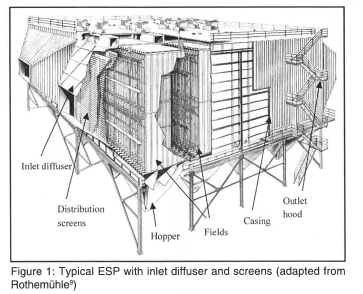
Due to space restrictions and cost limitations, long transitional ducts before Electrostatic Precipitators (ESP) are not practical in the design of modern power plants and therefore wide-angle transition pieces are commonly used in the flow path (as shown in Figure 1). Porous screens are inserted into the diffuser in order to improve the flow distribution entering the ESP. A near uniform flow distribution reduces peak velocities through the collection plates, which increase the treatment time and reduces the probability of particle re-entrainment.

 

 

CFD is used extensively in the design and optimisation of such systems although the methods used for the numerical simulation of distribution screens have not been well tested. This study investigates different methods that are proposed for the accurate simulation of these screens and reports on the findings. As part of the preliminary work, this study also investigates flow through wide-angle diffusers and the influence of numerical simulation parameters such as turbulence models and discretisation schemes on the accuracy of results.

 

2. Experimental setup

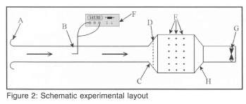
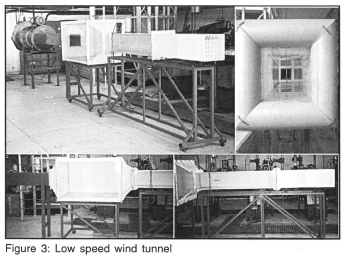
After consulting literature sources, the setup shown in Figure 2 and Figure 3 was chosen. An in-line configuration was used with an inlet bell mouth to ensure a well-developed flow profile. This design was based on experimental facilities proposed in literature ^7,8,14.

 

 

 

 

Where:

A: Inlet bell mouth

B: Pitot static tube measuring inlet velocity

C: Diverging diffuser

D. Distribution screen

E: Pressure tapping points in diffuser section

F: Digital pressure anemometer

G: Fan

H: Converging diffuser (reducer)

 

3. Uncertainty of experimental results

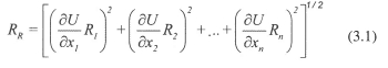
After the design and commissioning of the wind tunnel, the uncertainty and repeatability of experimental results were investigated. The method used is based on the uncertainty of the primary variables as shown in equation (3.1)³.

Where:

R_R is the uncertainty of the result

R_1...n is the uncertainty of the independent variables (x_1...n of the function U.

The uncertainty of measurement is below 3 percent for Reynolds numbers exceeding 1*10⁵ and increases to approximately 9 percent for Reynolds numbers in the region of 5* 10⁴. To reduce the uncertainty at low velocities, results were compared to literature^1,4,5 and it was found that the accuracy of empirical data is within 3 percent. The repeatability of experimental data was also investigated and a repeatability of 98.9 percent was achieved.

 

4. Preliminary conclusions from experimental results

Several different flow visualisation and measurement techniques were investigated, but it was found that flow visualisation supplies very limited empirical data, although it does assist the researcher in better understanding the flow distribution.

Apart from several minor problems, a major problem occurred when flow profiles were measured downstream from the diffuser. It was found that the flow profile was severely unsymmetrical. After considering factors such as measuring error, geometric imperfections of the wind tunnel and poor inlet flow distribution, it was found that this error is due to poor alignment of the different sections of the wind tunnel.

A simple alignment mechanism was devised in order to improve the alignment of the individual components and thus improve the symmetry of the flow profile through the wind tunnel. It was however not possible to ensure precise alignment with the equipment available. For this reason, all tests were conducted for both vertical and horizontal profiles. To minimise the influence that poor alignment may have on the uncertainty of experimental results, the average of both sets of data (i.e. six sets of results) was used for the correlation of numerical data.

 

5. Flow through wide angle diffusers

Before attempting to simulate screens inside the diffuser, the influence of numerical solution parameters such as turbulence models and discretisation schemes on the simulation of flow through wide-angle diffusers was investigated. Two diffuser angles were chosen that would envelope industrial applications, i.e. 60° and 120° inclusive angles.

Measurements consisted of a horizontal and vertical traverse at different positions inside the diffused section and at a single Reynolds number in the turbulent region (approximately 2.5e⁵). Schubauer et. al.¹⁰ and Moore et. al.⁶ found that variations in Reynolds number and aspect ratio seem to have little effect on the flow regime for the range of aspect ratios normally encountered and for all Reynolds numbers in excess of a few thousand.

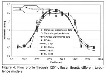
The commercial CFD code Star-CD Version 3.15 for Windows¹² was used for this study. Figure 4 shows comparative results between CFD simulations using the first order upwind differencing (UD) discretisation scheme with different turbulence models compared to the experimental data. The UD scheme does not predict the flow profile very accurately and the difference between the turbulence models is marginal.

 

 

From Figure 5 it can be seen that the higher order discretisation schemes show a better correlation with the experimental data. It should however be noted that results for the 60° diffuser did not compare as well as for the 120° diffuser. Only the turbulence models included as standard in Star-CD Version 3.15 could be tested.

 

 

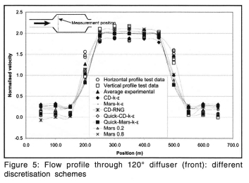
The standard high Reynolds number k-ε turbulence model shows reasonably good correlation with the experimental results. The RNG turbulence model, which is expected to predict flow separation and reattachment better than the k-ε model¹², combined with the CD discretisation scheme does not show improved results in this instance. It is however expected that advanced turbulence models (such as v²-f) could show improved results. Based on these results and the available models, it was concluded that the standard high Reynolds number k-e turbulence model should be used in conjunction with the MARS discretisation scheme as generally recommended by Computational Dynamics.

 

6. Theoretical approach

Three different approaches were investigated during this study. These included:

□ The porous medium approach

□ The momentum sink approach and

□ The porous baffle approach

Variable porous medium approach

The perpendicular free area ratio (FAR) was calculated with:

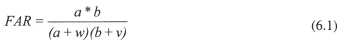
Where: (see Figure 6)

 

 

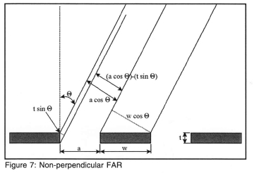
This methodology was then expanded to include non-perpendicular angles in the calculation of the FAR as shown in Figure 7 and equation (6.2).

 

 

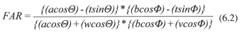
Since the FAR cannot be used to calculate the resistance across a certain screen directly, it is required to find a relation between the FAR of the screen and the resistance coefficient (K). The latter is defined by the following equation:

Where:

∆P is the pressure drop (Pa)

ρ density

v velocity

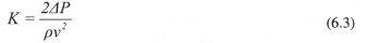
From literature^1,4,5, it was found that the relation between K and FAR can be defined by the following equation as shown in Figure 8:

 

 

 

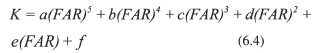
Where:

a =-4444.8297

b =13200.9818

c =-15548.5414

d =9129.9442

e =-2705.0564

f =331.5113

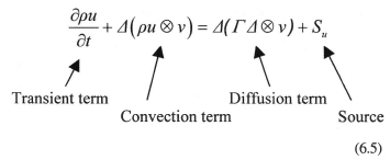
After calculating the variable value of K, it is required to implement this value into the CFD code. This was done by using the source term in the Navier-Stokes equation^2,15:

(see equation 6.5 overleaf)

Ignoring convective acceleration and diffusion, the porous medium model reduces to Darcy's law (assuming plug flow)¹²:

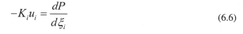
Where:

dP: Pressure drop (Pa)

>: (i=l, 2, 3) represents the mutually orthogonal orthotropic directions

K_i|: Permeability

u_i: Superficial velocity in direction > (m/s)

The permeability K¡ is assumed to be a quasi linear function of the superficial velocity magnitude \u\ of the form:

It should be noted that the simplified momentum equation is valid provided that:

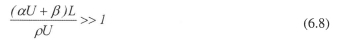
Where L and U are characteristic overall dimensions of the distributed medium and a characteristic velocity through it respectively.

Combining equations (6.6) and (6.7), the pressure gradient that is calculated in the momentum equation by Star-CD across a porous medium is represented by:

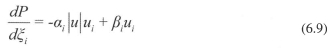
Assuming that the velocity is always positive, that d> is some length dL and that ß→0, equation (6.9) can be written as:

For unit length, the equation for pressure drop becomes:

Combining equations (6.11) and (6.3), the value of α, is now directly related to the variable resistance coefficient (K_v):

The value of a, now being a function of the flow incidence angle and screen geometry, is then used in the standard calculation of the pressure drop across the screen in the direction of the flow.

User defined functions (Subroutines)

The calculated variable resistance coefficient was implemented through the Star-CD subroutine called poros1.f. It was required to obtain the flow properties of the upwind neighbour cell in order to calculate the approach velocity. This was done by creating a neighbour cell listing using the posdat.f subroutine. Additional global vectors (common blocks) were required and these were defined through a separate user file. All geometric inputs (defining the screen specification) were also implemented through a separate user file. These files were called automatically from the subroutines and therefore the user does not have to access the main subroutines. Calculated variables were stored in scalars using the scalfn.f subroutine to allow access to the scalars in Prostar for post processing.

Momentum sink approach

It was found that the physical properties of some screens did not conform to the limitation imposed on the use of porous media as shown in equation (6.8). In such cases, it was required to use a negative momentum source term (momentum sink) approach. This approach was introduced through the sormom.f subroutine and could be implemented either implicit or explicit^12,13:

If implemented using S1, the momentum sink is explicit, i.e. it is included only in the source term on the right hand side of the Navier-stokes equation (6.5). When using S2, the momentum sink is again multiplied with the velocity magnitude by the code thus forming part of the convection term and not the source as shown in equation (6.5). With the explicit approach being included through the source term, it was expected to be less stable than the implicit approach¹².

With the implicit approach, it was found that the pressure drop across the momentum sink region was underestimated when compared to literature^1,4,5. A simple test case was created and results showed that the porous medium approach and explicit momentum approaches accurately predicted the pressure drop. Upon further investigation, it was found that the average velocity through the implicit momentum sink region was lower than the average approach velocity (see Figure 9).

 

 

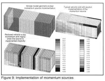
Since this velocity is again used in the Navier-Stokes equation to calculate the momentum sink through the convection term, the pressure drop is underestimated. This issue was discussed with CD-adapco and it was explained that this phenomenon is due to the implementation of the Rhie and Chow interpolation^2,12,15. This does however not solve the under prediction of the pressure drop. In order to overcome this problem, a correction factor (CF) was introduced:

CF=Upwind neighbour cell velocity/Local velocity (see Figure 9 overleaf)

Since the neighbour cell velocities were already available from the common blocks, it could easily be retrieved in order to correct the under prediction of the pressure drop. It was found that the implementation of the correction factor to the implicit approach resulted in an accurate prediction of the pressure drop. Due to the improved accuracy of the implicit approach (with the implementation of the correction factor) and the expected numerical stability, it was decided to include the implicit approach in this study.

The conventional porous medium approach

Schmitz et. al.¹¹ investigated the use of conventional porous media to simulate screens in diffusers. With this approach, equation (6.10) is used to calculate the value of α based on the theoretical pressure drop for a certain screen. This value is applied uniformly across the porous medium not accounting for changes to the FAR due to a change in the angle of incidence.

The variable porous baffle approach

The possibility of using a porous baffle with a variable resistance coefficient defined through user coding was also investigated. It was found however that a baffle boundary could not be defined in Star-CD Version 3.15 through user coding. The alpha and beta values can only be defined as constant values. Since this is not a standard function, variable baffle resistance values could not be included in this study.

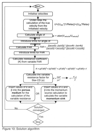
Solution algorithm

Figure 10 shows the simplified solution algorithm for the calculation of variable resistances using both the porous medium and momentum sink approaches.

 

 

The conventional porous baffle approach

A conventional method of modelling screens in a diffuser is by using a simple baffle (local planar resistance) to represent the screen. The pressure drop implemented in the solution is calculated by¹²:

Where:

dP: Pressure differential across the porous baffle (Pa)

ρ: Density of the fluid (kg/m³)

αUser defined variable (kg/m⁴)

ß: User defined variable (kg/m³.s)

u: Perpendicular superficial approach velocity (m/s)

Assuming that the velocity is always positive, that and combining equation (6.14) with (6.3), it can be shown that:

A variation of this approach where the value of a, is again divided by 2 was first suggested by Schmitz et. al.¹¹:

Although there is no mathematical reasoning behind this approach, results did show a rather good correlation with empirical data for the 50 percent FAR screens. For this reason it was decided to also include this approach in this study.

 

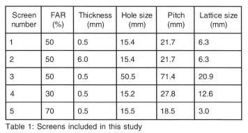
7. Screens included in this study

Five different screens were tested in both the 60° and 120° diffusers. Screens were chosen to test specific phenomena:

□ The influence of the thickness of the screen.

□ The influence of the screen FAR.

□ The influence of the ratio between the lattice width of the screen holes to the size of the flow area (w/D_H).

Where:

□ Hole size refers to the size of the hole in both vertical and horizontal directions (i.e. square holes).

□ Pitch refers to the length between successive lattices.

□ Lattice size refers to the size of the solid parts of the screen (w).

 

8. Discussion of experimental results

In order to show general trends from the experimental data, the six traverses measured for the vertical and horizontal flow profiles were averaged and were compared to results from the other screens. Figure 11 and Figure 12 show these comparisons for the 60° and 120° diffusers respectively in the central diffuser position.

 

 

 

 

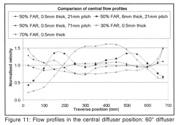
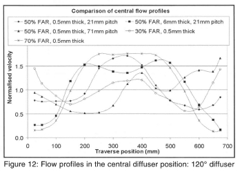
It can be seen that the flow profile is reversed as the screen resistance increases. This is evident for both the 60° and 120° diffusers. The influence of the screen thickness can also be seen when comparing the 0.5mm 50 percent FAR screen with the 6mm screen. The thicker screen shows very similar results to the 70 percent FAR screen, especially for the 120° diffuser.

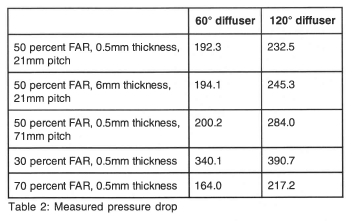
Table 2 shows the measured pressure drop for the screens tested in both diffusers. It can be seen that the pressure drop did not increase significantly with an increase in screen thickness. A change in the pitch did however result in a marginal increase in resistance. As could be expected, a change in FAR has a major influence on the pressure drop across the screens.

 

 

 

9. Discussion of CFD results

Figure 13 shows the numerical mesh used for the CFD simulations. The mesh was refined along the walls in order to obtain the correct y+ values. Further refinement was required around the screen to improve the stability of the numerical algorithm. Initial simulations were conducted with a large atmospheric pressure inlet boundary. It was found however that this boundary introduced significant numerical instability. For this reason, the inlet boundary profile as measured in the wind tunnel was implemented through a user-defined function.

 

 

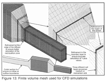
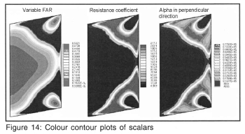
Figure 14 shows colour contour plots of typical scalars calculated through subroutines in the position of the screen. The ability to view the calculated scalar values, assisted in understanding the behaviour of the subroutines and also in the debugging of the code.

 

 

60° diffuser

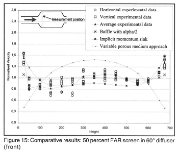
From Figure 15 it can be seen that both the momentum sink and porous baffle approaches show a reasonably good correlation with experimental data for the 50 percent FAR screen with 0.5mm thickness. The variable porous medium approach however fails to predict the reversal of the flow profile.

 

 

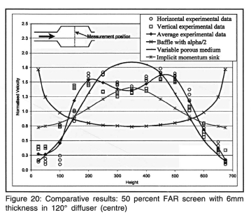
With the thickness of the screen increased however, it can be seen from Figure 16 that only the porous medium approaches show a reasonable correlation with experimental data. The lower velocities in the central region are however not captured and the velocities are over predicted.

 

 

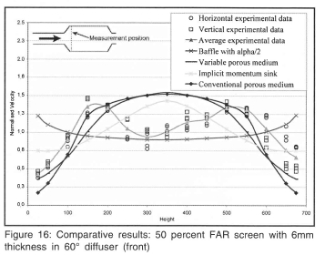
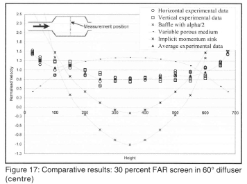
Figure 17 shows that none of the approaches accurately predicted the flow profile downstream of the high resistance (30 percent FAR) screen. Both the baffle and momentum sink approaches severely over predicted the flow near the walls of the diffuser.

 

 

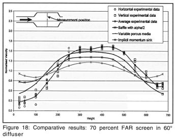
With the low resistance of the 70 percent FAR screen, it can be seen from Figure 18 that the variable porous medium approach shows the best correlation with the experimental data.

 

 

120° diffuser

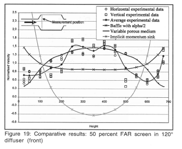
It was found that the numerical results did not show very good correlation with the experimental data from the 120° diffuser. Although the porous medium approach showed similar trends, it failed to predict the flow profile precisely as shown in Figure 19 and Figure 20.

 

 

 

 

Similar to the 60° diffuser, it was found that the numerical approaches did not accurately predict the flow profiles down-stream of the high resistance screen (30 percent FAR) or the screen with increased thickness.

Predicted pressure drop

It was found that the pressure drop was generally under-predicted by approximately 25 percent. In some instances however the pressure drop prediction was quite accurate (within 10 percent).

 

10. Mesh independence

To test the influence of mesh (grid) refinement, the mesh was refined once in all orthogonal directions (i.e. 2*2*2 refinement) thus resulting in eight times as many cells as the original mesh. This refinement resulted in a mesh containing 1.2e6 cells for the relatively small section of geometry as shown in Figure 13.

Results with the MARS discretisation scheme revealed a peculiar unsteady flow pattern as shown in Figure 21. These tests were repeated with the UD discretisation scheme and it was found that the unsteady flow pattern disappeared. The results obtained with the refined model and the MARS scheme may be due to the extremely high level of refinement coupled to the highly turbulent nature of the flow downstream of the diffuser. Due to the sensitive nature of information regarding the MARS scheme, very little is known about the characteristics of the scheme. It is believed however that the unstable behaviour may be due to un-boundedness introduced by the downstream component of the MARS scheme, being a higher order discretisation scheme.

 

 

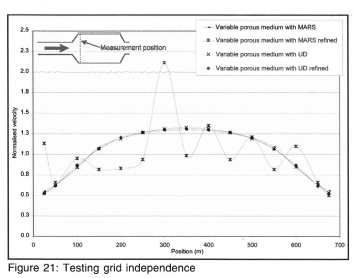
Further research would be required to better understand these results. It can however be seen that both the coarse and fine mesh results with the UD scheme compares well with results from the coarse MARS scheme thus confirming grid independence.

 

11. Conclusions and recommendations

□ It was concluded that the experimental facility was accurate within 3 percent with an uncertainty not exceeding 3 percent for Reynolds numbers in excess of 1e⁵ and that results were 98.9 percent repeatable.

□ Experimental testing is not easily accomplished and even with a relatively simple geometry such as the one used in this study, small imperfections, such as alignment of components, can result in significant errors in measurement.

□ From the simulation of flow through wide-angle diffusers, it was found that the turbulence model did not have a significant influence on the results. This can possibly be contributed to the fact that all of these models assume isotropic turbulence. The influence of the discretisation scheme was more significant. Based on the results obtained, it was recommended that the standard high Reynolds number k-ε turbulence model combined with the MARS discretisation scheme be used for this type of application. It should however be noted that all the turbulence models available in this version of Star-CD are derivatives of the k-e model. It is therefore suggested that this study be expanded to include more advanced turbulence models such as v²f.

□ With the low resistance of the 70 percent FAR screen, the variable porous medium approach shows the best correlation with the experimental data.

□ Furthermore, it was found that none of the CFD results predicted the flow profile very well for the very high resistance screen (i.e. 30 percent FAR). The momentum sink approach showed the best prediction, although the higher flow near the walls were over estimated. Further research would be required to improve on the predicted CFD results with higher resistance screens.

□ For the 50 percent FAR screen, it was found that no single model accurately predicted the flow profile through both diffusers. With the 120° diffuser the variable porous medium approach was more accurate while the porous baffle approach (with a/2) showed a better correlation with experimental data of the 60° diffuser.

□ With the 120° diffuser, only the variable porous medium approach showed similar trends to the experimental data although it failed to predict the flow profile precisely.

□ It was found that the total pressure drop was under estimated by an average value of approximately 25 percent for the screens tested. In some cases however the predicted pressure drop differed by less than 10 percent from the experimental data although the tendency still was to under predict the pressure drop.

□ The experimental procedures focused on the flow distribution downstream of the screen. Based on results from this study, it was recognised however that the flow distribution between the diffuser inlet and the screen has a major influence on the distribution downstream of the screen. To improve the accuracy of numerical models, it would be required to improve the experimental procedures in order to accurately measure the flow profiles just upstream of the screen and compare this empirical data with results from the numerical methods.

□ In general, it can be concluded that at least one of the three approaches tested in this study showed an improved prediction of the flow field downstream of the screen for thin screens with FAR's exceeding 50 percent when compared to conventional methods. Thin screens are defined as having a ratio between lattice size and thickness exceeding a value of 10. For screens with increased thickness or higher resistance (i.e. 30 percent FAR), it was found that the CFD models did not predict the flow profile or pressure drop very well.

□ Although a single numerical approach could not be found that accurately predicted the flow profile for all screens tested, results from this study serves as a foundation for further research into this field.

 

12.Acknowledgements

□ The authors wish to thank the following people who contributed to this study:

□ Mr. J. Nel and Mr. S. Bolatti for their assistance during the design, testing and commissioning phase of the project.

□ Prof. B. Skews (of Wits University) for his assistance and guidance.

□ Dr. J. Hoffmann and Mr. C. Viljoen for their assistance in the editing.

□ For financial support: The Vaal University of Technology, The National Research Foundation (NRF) and Eskom TSI, specifically Mr. D. Gibson.

 

References

1. Blevins, R.D. 1984.Applied Fluid Dynamics Handbook. New-York: Van Nostrand Reinhold Company Inc.         [ Links ]

2. Fertiger, J. H. and Peric, M. 2002. Computational methods for fluid dynamics. 3^rd revised edition. Springer: Berlin, Germany. Idelchick, I.E. 1986. Handbook of Hydraulic Resistance. 2^nd Ed. Translated by E. Fried, Washington.

3. Holman, J.P. 1989. Experimental methods for engineers. 5^th Ed. Singapore: McGraw-Hill, ISBN 0-07-029601-4.

4. Idelchick, IE. 1986.Handbook of Hydraulic Resistance. 2^nd Ed. Translated by E. Fried, Washington.

5. Miller, D.S. 1978. InternalFlow Systems. BHRA Fluid Engineering Series, BHRA Fluid Engineering, vol 5.         [ Links ]

6. Moore, C.A., Kline, S.J. 1958.Some effects of vanes and of turbulence in two-dimensional wide-angle subsonic diffusers. National advisory committee for aeronautics (NACA), Technical note no. 4080.

7. Pinker, R.A., Herbert, M.V. 1967. Pressure loss associated with compressible flow through square-mesh wire gauzes. Journal of Mechanical Engineering, Sei. 9:11-23.         [ Links ]

8. Plint, MA., Böswirth, L. 1978.Fluid mechanics: A laboratory course. London and High Wycombe: Charles Griffin & Company.         [ Links ]

9. Apparatebau Rothemühle General Sales and Marketing brochure, 1999.

10. Schubauer, G.B. and Spangenberg, W.G. 1948. Effect of screens in wide-angle diffusers. National advisory committee for aeronautics (NACA), Technical Note no. 1610.

11. Schmitz, W., Pretorius, L., van Niekerk, A. and Lalla, T. J. 1998. Modelling of screens within industrial flow applications. In Proceedings of the 2^nd South African Conference on Applied Mechanics (SACAM). 13-15 January, 1998. Vol. 2, pp. 865-875.

12. Star-CD Methodology manual, Version 3.15, 2001. Methodology pp 1.1-10.2, Computational Dynamics LTD, Latemer Road, London, United Kingdom.

13. Star-CD User guide, Version 3.15, 2001. Computational Dynamics LTD, Latemer Road, London, United Kingdom.

14. Taylor, G.I. and Davies, R.M. 1944. The aerodynamics of Porous Sheets. Reports and Memoranda, No. 2237.

15. Versteeg, H.K, Malalasekera, W„ 1995. An Introduction to Computational Fluid Dynamics The Finite Volume Method. Malaysia: Longman Group Ltd. ISBN: 0-582-21884-5.         [ Links ]