Transformer Thermal Modelling, Load Curve Development and Life Estimation

 

 

CB Holtshausen

At time oí doing the research, the author was at Powertech Transformers (Pty) Ltd, 1 Bultenkant Street, Pretoria West, 0183. Currently at Eskom Holdings (SOC) Ltd, Sunninghill, 2157. E-mail: holtshcb@eskom.co.za

 

 

---

ABSTRACT

This paper presents an algorithm for transformer load curve development. In addition, the paper examines the effect of thermal time constants and insulation paper, to loading time limits and loss-of-life. The applied thermal model is based on the 'exponential time constant' analogy for transformer top-oil temperature and hot-spot temperature. An overview of the theoretical basis for the underlying thermal and aging model is given. The derived equations are applied in a MATLAB environment; whereafter a case study is presented. Loading time results are compared to those from a commercial software package, and new results presented for the corresponding effect on paper insulation life. The difference in permissible duties for design-specific to default time constants specified in IEC60076-7:2005 are shown to be significant.

Additional keywords: Transformer; Thermal model; Load curve; loss-of-life; Overloading; Temperature

---

 

 

Nomenclature

Roman

C Thermal capacity

D, d Difference operators

Κ Load factor [p. u. ]

L Loss-of-life [s]

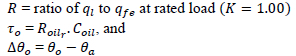
R Ratio of load loss (q_ι) to no-load loss at rated load (q_fe )

V Relative aging rate

c Conductor specific heat , 390 for copper

g Winding-to-oil gradient at load considered [K]

k Correction factor

m Mass [kg]

η Time step counter

q Loss at load considered [W]

t Time [s]

x Oil exponent (empirical)

y Winding exponent (empirical)

Greek

Δ Temperature rise [K]

θ Temperature [°C]

τ Time constant [s]

Subscripts

11,21,22 Empirical factors A Core and coil assembly Τ Tank and fittings a Ambient

h Hot-spot

0 Top-oil

om Mean-oil

r Rated load (K = 1.00)

s Standard paper (Non-thermally upgraded)

su Supplied

u Thermally upgraded paper

w Winding

 

1 Introduction

The temperature status of a transformer is vital during operation and even more so, during overloading conditions¹. This is directly contributed to the relation between heat and insulation breakdown, as related by the empirically valid Arrhenius equation². As insulation breakdown is considered to be a major cause in the reduction of transformer life expectancy, the importance in modelling the overloading condition is growing³.

Of late, the concept of 'planned loading beyond nameplate during normal operation' has gained notable interest. This is because planned loading operations could considerably reduce costs without affecting reliability^{4, 5}. As load curves relate the load factor to the time for which the transformer can be overloaded, they can be a useful tool in implementing planned loading operations, allowing the utility to gain more from their transformers.

The current loading guide standards stipulate a thermal model which is fundamentally based upon the relational properties of exponential equations. In its differential form, this model allows for discrete and dynamic modelling of temperatures over time³. By implementing these equations in a programming environment and applying an algorithm, these equations can be extended to estimate loading curves for planned loading operations.

The intent of this paper is to provide a methodology on how the loading guide standards might be applied to determine allowable transformer loading. In addition, the effects of the variation of thermal constants to loading time and the selection of winding insulation to the aging rate are investigated.

 

2 Transformer modelling

2.1 Exponential time constant analogy

Transformer thermal response is a subject that has been addressed in various studies. The standards and literature, at first, are seemingly confusing and unclear^{6, 7}. This confusion arises from the fact that two similar, but fundamentally independent models have developed following two different approaches, namely the 'exponential time constant' analogy and the 'thermal-electrical' analogy^6,7. In the following overview, only the equations for the exponential time constant analogy will be given. The equations for the thermal-electrical analogy can be found in the Appendix.

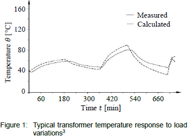
The temperature response of a transformer to varying load current can be represented with rising and falling exponential functions. As such, the exponential time constant analogy is derived by applying heat transfer principles in conjunction with exponential curve fitting methods⁶. This 'fitting' of the solution curve to represent the temperature response is depicted in figure 1 for a typical load cycle.

 

 

However, the response of top-oil or hot-spot temperature rises to a step change in load current is not a true exponential function and therefore requires the solution curve to be 'corrected'. This is achieved by applying the necessary correction factors to the thermal time constants as is evident in equation 1^{3, 7}.

For the purpose of modelling the temperature response in a discretely time dependent manner, the exponential form of the equations are not sufficient. This is due to the inherent exponential constant e and the need of a sufficiently large step function³. For this reason, differential equations are inferred from the fundamental equations, which are in-turn, directly obtained from the exponential time constant analogy⁶.

The differential equation inferred from the exponential equation for the top-oil is as follows³:

It should be noted that the equations for the hot-spot calculations are not given as they are completely analogous to that of the top-oil⁷.

2.2 Difference solution

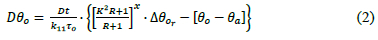
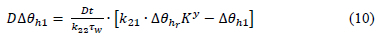
For the purposes of easily solving the models discussed, the equations are reformulated to that of the difference solution method. This is done by introducing the difference operator D, indicating a small change in the accompanying variable as is represented in equation 2^{3, 7}. The full set of difference equations necessary, to solve for both the top-oil and hot-spot can be found in section 3.

The difference equation corresponding to equation 1 is:

2.3 Thermal time constants

As discussed in section 2.1, the exponential time constant analogy implies the use of time constants to characterise the temperature response for a specific thermal system. Default values for these parameters can be found in the loading guide standards. Alternatively, the equations in this section can be used to determine more accurate design-specific constants³.

The winding time constant in minutes at the load considered is:

The average oil time constant in minutes at the load considered is:

For an Oil Natural Air Natural (ONAN) cooling type the thermal capacity is:

2.4 Relative aging and loss-of-life

Transformer loss-of-life estimation is based on the degradation of the insulation tensile strength to half that of the initial tensile strength. Beyond this limit the chance of dielectric failure of the conductor insulation is considerably high⁸. The following method is based on the latter quantitative criterion in combination with the Arrhenius equation³:

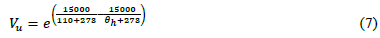
Using the hot-spot temperature from equation 13, the relative aging rate for standard paper is:

For thermally upgraded paper the relative aging rate is:

The loss-of-life can then be calculated using:

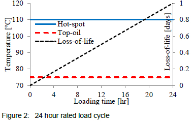
To illustrate transformer loss-of-life, figure 2 was plotted using the equations covered in section 3. Note that at rated load the hot-spot temperature corresponds to the value in equation 7. Also, note that for a 24 hour rated load profile the temperature response remains flat and the loss-of-life amounts to one day as per the definition in International Electrotechnical Commission (lEC) 60076-7:2005³.

 

 

The full set of difference equations necessary to solve for the aging rate and loss-of-life can be found in section 3.

 

3 Transformer modelling

In order to solve the transformer thermal model and relating loss-of-life, as discussed in section 2, all the relevant equations are reformulated to difference equations. This section provides the remaining set of equations needed for successful implementation in a computer program.

In the case of the top-oil (see equation 2) at each time step, the n^th value of Dθ_o is calculated from the (n - 1)^th value using^{3, 7}:

The hot-spot temperature response is solved in the same way as for equation 9, but for the following two difference equations:

And,

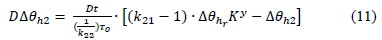
Where:

The separation of Δθ_h(η) into two separate difference equations represents two separate physical phenomena. Note that equation 10 contains the winding time constant while equation 11 contains the oil time constant τ₀ . The first equation represents the faster fundamental hot-spot temperature rise which does not consider the oil flow passing it³. The second equation represents the slower effect of the oil flow passing the hot-spot³.

Finally, the hot-spot temperature is solved by adding the temperature rise of the hot-spot to the absolute top-oil temperature at the nth time step:

The relative aging rate at the nth time step is solved using:

Again, the difference equation for loss-of-life is solved similarly to equation 9:

It is important to note that in order to get an accurate temperature response; the time step should not be greater than half the smallest time constant in the thermal model³.

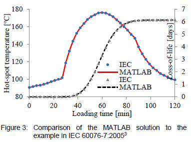
An application of the solution routine discussed is presented in figure 3. The solution routine was implemented in MATLAB and compared to an example provided in Annex C of IEC 60076-7:2005³. The logic flow for the solution routine is also depicted in a section of figure 4, highlighted by the segmented square.

 

 

 

 

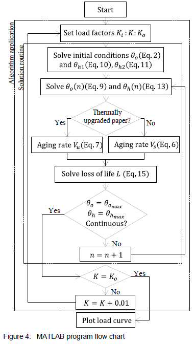
4 Algorithm application

The previous section introduced a solution routine that can be applied to determine a single thermal response given the appropriate inputs and initial conditions. This routine can be extended by applying an algorithm to solve the same routine multiple times.

The algorithm requires that an initial load factor K_i be selected and that this load factor be increased by a load step Κ for each completed solution routine. The conditions for halting the solution routine play an important role and are defined as:

• Reaching the top-oil limit, θ_o = θ_οmax

• Reaching the hot-spot limit, θ_h = θ_hmax

• Achieving a continuous temperature response, θ_o(η) = θ_o(η - 1) or θ_h(η) = θ_h(η - 1)

When the solution routine halts, the load factor Κ is increased and the solution routine is repeated for the new loading factor. This is done until K_o is reached. To illustrate, figure 4 presents the logic flow for the algorithm in the section highlighted by the segmented square.

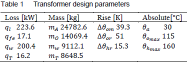
The algorithm was finally applied to develop a loading curve for a 40MVA, 132/11kV, ONAN, three phase power transformer with design parameters as shown in table 1 below:

 

 

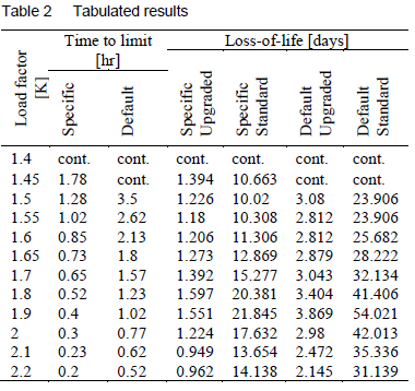
5 Results

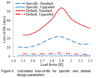
Using the program shown in figure 4, a loading curve was computed for both default design parameters and specific design parameters. The default parameters were selected based as per IEC 60076-7:2005³, while the specific parameters were determined using the equations in section 2.3. Furthermore, the resulting loss-of-life for both standard paper and thermally upgraded paper was computed.

The results are portrayed in figures 5 and 6 and table 2. For comparison, the results for the load curves are presented against those obtained from a commercial software package used by the manufacturer. A time step size Dt of 1 minute was used with a load factor step size K of 0.01 per unit. The average solution time for both computational runs was 0.36 seconds for K_i = 1 to K_o = 2.2 per unit.

 

 

 

 

 

 

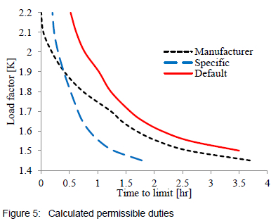
6 Conclusions and recommendations

Looking at figure 5, it is clear that the solution curve trend for the default design parameters resemble that of the manufacturer. As such, it is reasonable to assume that the manufacturer's results are based on similar constants to that found in IEC 60076-7:2005³. Results obtained for the default solution are less conservative to those of the manufacturer. This could possibly be attributed to safety margins used by the manufacturer. However, further investigations are required to explore other possible causes.

Conversely, the design-specific parameter results are conservative as is evident to those of both the default and manufacturer solution. This is attributed to the thermal time constants being derived from design characteristics of the actual transformer unit. The conservatism, however, could be coincidental and could vary pending the transformer under consideration. Additional case studies like the one presented in this paper are required to confirm this.

In addition, the effect of thermally upgraded paper greatly outplays that of standard paper with regards to loss-of-life as presented in figure 6. Thermally upgraded paper shows an improved loss-of-life of up to 15 times that of standard paper under the same conditions.

In conclusion, the effects of the thermal time constants and the selection of paper insulation play an important role in assessing the permissible loading duties of transformers. The methodology presented in this paper seems to be appropriate to determine load curves for planned loading operations.

It is recommended that the relevant parameters for overloading conditions be obtained from manufacturers for the development of optimal load curves, as these could have a significant impact on transformer life estimation.

 

Acknowledgements

The work presented here was done at the Technology Department of Powertech Transformers (Pty) Ltd, Pretoria West, 0183. This work has been presented at the 2014 POWER-GEN Africa conference under the title "Transformer Thermal Modelling and Load Curve Development". 1 would like to thank Mr Johan Haarhoff and the management of Powertech Transformers for their support.

 

References

1. Susa D, Dynamic Thermal Modelling of Power Transformers, PhD thesis, Helsinki University of Technology, 2005.         [ Links ]

2. Connors KA, Chemical Kinetics, VCH Publishers, 1990.

3. International Electrotechnical Commission, Part 7: Loading Guide for Oil-1mmersed Power Transformers, 1EC 60076-7. 2005-12.

4. Franchek MA and Woodcock DJ, Life-cycle Considerations of Loading Transformers Above Nameplate Rating, 65^th Annual International Conference of Doble Clients, 1998.

5. Strongman B and Harris K, Loading of Power Transformers: Reducing Costs Without Affecting Reliability, Burns & McDonnel TechBriefs, 2001, 4, 4-6.         [ Links ]

6. Swift S, Fedirchuk D and Zhang Z, Transformer Thermal Overload Protection - What's 1t All About?, 25^th Annual Western Protective Relay Conference, Spokane Washington.

7. Swift G, Molinski TS and Lehn W, A Fundamental Approach to Transformer Thermal Modelling, IEEE Transactions on Power Delivery, 2001, 16(2), 171-175.         [ Links ]

8. Chiulan T and Pantelimon B, Theoretical Study on a Thermal Model for Large Power Transformer Units, Proceedings of World Academy of Science, Engineering and Technology, Vol. 22, 2001, 440-443.         [ Links ]

9. Nawzad R, Short-Time Overloading of Power Transformers, ABB Corporate Research, Royal Institute of Technology, Stockholm, Sweden, 2011.

10. Jauregui-Rivera L and Tylavsky DJ, Acceptability of Four Transformer Top-oil Thermal Models - Part 1: Defining Metrics, IEEE Transactions on Power Delivery, 2008, 23(2), 860-865.         [ Links ]

 

 

Received 4 July 2014
Revised form 17 February 2015
Accepted 17 March 2015

 

 

Appendix

Thermal-electrical analogy

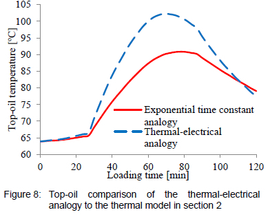
The basis of this approach is that of a thermal-electrical circuit, as shown in figure 7⁷. This model followed from the need for an electrically intuitive analogy in a predominantly electrical environment and is the subject of several relatively recent studies^{1, 8, 9, 10}.

 

 

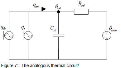
Favourably, differential equations follow directly from the RC-circuit analogy⁷. Also, because the step change is no longer represented by an exponential function the solution curve needs no correction factor⁷.

The differential equation for the equivalent circuit shown in figure 1 is:

If we define,

then equation 16 reduces to:

Note that the structure of equation 1 and equation 17 are very similar albeit their fundamentally different origins. These similarities carry through to the difference equations.

The difference equation corresponding to equation 17 is:

Importantly, the present standards rely only on the exponential methodology. Still, they also include differential equations inferred from the exponential response⁷. This reformulation of the exponential time constant analogy to differential equations, as well as the similarity of the equations, account for most of the confusion mentioned in section 2.1.

As evident in figure 8, the different thermal models do vary in accuracy and as such, a lot of recent work has gone into comparing and improving the thermal models. See Dejan¹ and Rivera et al¹⁰.